KMV Model

Published on :

21 Aug, 2024

Blog Author :

Edited by :

Reviewed by :

The KMV model estimates default possibility and probable loss for companies. It combines elements from the structural approach, which focuses on the firm's capital structure and asset value, with a reduced-form approach that considers the probability of default as an exogenous variable. The purpose of the KMV model is to provide a quantitative framework for assessing and managing credit risk.

By estimating the (probability of default) PD and (loss given default) LGD, the model helps investors, lenders, and financial institutions evaluate the creditworthiness of borrowers and make informed decisions regarding lending, investment, and risk mitigation strategies. The KMV - Kealhofer Merton Vasicek model is important because it offers a comprehensive and theoretically sound approach to credit risk assessment.

What Is KMV Model?

The KMV model combines structural and reduced-form elements, integrating market-based information and company-specific data to provide a comprehensive framework for credit risk assessment.
In addition to (probability of default) PD, the KMV model also estimates the expected loss given default (LGD), representing the potential loss in the event of default.
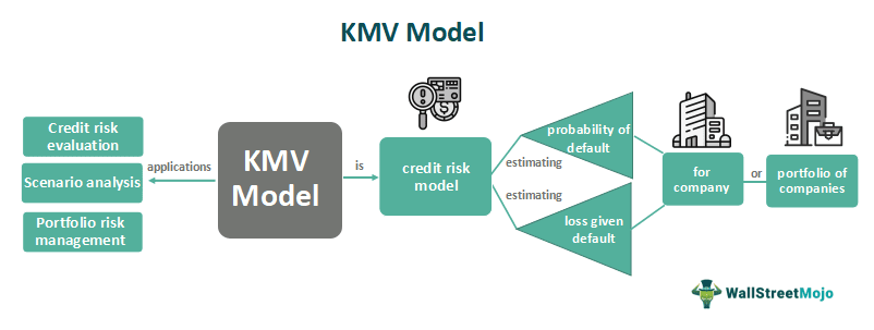
The KMV model finds applications in credit risk evaluation, portfolio risk management, pricing of credit-sensitive instruments, stress testing, scenario analysis, and risk-based capital allocation.
It enhances risk management practices and facilitates informed decision-making in credit-related activities.

KMV Model Explained

The KMV (Kealhofer Merton Vasicek) model is a credit risk model that Kealhofer, Merton, and Vasicek developed to estimate the probability of default (PD) and the expected loss given default (LGD) for a company or a portfolio of companies. It incorporates market-based information and company-specific financial data to estimate the likelihood of default and potential losses. This enables users to better understand and quantify credit risk exposures, leading to improved risk management practices and more effective capital allocation in credit-sensitive activities.

The KMV model considers the firm's capital structure and asset value in the structural approach. It assumes that a firm defaults when its liabilities exceed the value of its assets. By modeling the dynamics of the firm's assets and liabilities, the KMV model estimates the likelihood of default based on the distance between its asset value and default threshold.

The reduced-form approach, on the other hand, treats the probability of default as an exogenous variable. It models the default process as a stochastic event determined by macroeconomic factors, market conditions, and company-specific characteristics. The KMV model incorporates these factors to estimate PD and LGD.

It provides a quantitative framework that allows users to evaluate borrowers' creditworthiness, make informed lending and investment decisions, and develop effective risk management strategies. By integrating market-based information and company-specific data, the KMV model enhances the understanding and quantification of credit risk, leading to improved risk management practices in the financial industry.

How To Calculate?

The calculation of the KMV model involves estimating the probability of default (PD) and expected loss given default (LGD). Let us look at the steps involved:

Collect company-specific data: Gather financial information about the company, including its capital structure, asset values, liabilities, and relevant market data. This may include financial statements, market prices, interest rates, and other relevant inputs.
Estimate asset value: Use the company's financial data and market information to estimate the value of its assets. This can be done using various methods such as discounted cash flow (DCF) analysis, market multiples, or other valuation techniques.
Determine default threshold: Set a threshold value that represents the point at which the company is considered to default. This threshold can be determined based on the company's debt obligations, financial covenants, or credit rating standards.
Calculate distance to default: Measure the distance between the estimated asset value and the default threshold. This distance is typically expressed in standard deviations, representing the company's risk of default.
Estimate PD: Using statistical techniques, map the distance to default to a corresponding probability of default (PD). This step involves using historical data or market-based indicators to establish a relationship between the distance to default and the likelihood of default occurring.
Determine LGD: Estimate the expected loss given default (LGD), representing the potential loss in the event of default. LGD can be derived from historical data, industry benchmarks, or credit rating agencies' information.

Application

Let us look at key applications, including:

Credit risk evaluation: Model provides a quantitative framework for assessing credit risk. It helps investors, lenders, and financial institutions evaluate the creditworthiness of borrowers by estimating the probability of default (PD) and expected loss given default (LGD). This information is crucial for making informed decisions regarding lending, investment, and risk mitigation strategies.
Portfolio risk management: It can be applied to assess credit risk at a portfolio level. By estimating the PD and LGD for each company in a portfolio and aggregating the results, portfolio managers can gain insights into their portfolios' overall credit risk exposure. This allows for effective risk management, diversification strategies, and the optimization of capital allocation.
Stress testing and scenario analysis: It enables stress testing and scenario analysis by providing a framework to assess the impact of adverse market conditions on credit risk. By adjusting inputs, such as asset values or macroeconomic factors, users can evaluate the resilience of portfolios and companies to various stress scenarios.

Significance

Let us look at key aspects that highlight its significance:

Enhanced risk measurement: The KMV model provides a comprehensive framework combining elements from structural and reduced-form approaches to credit risk. This integration allows for a more accurate and robust estimation of the probability of default (PD) and expected loss given default (LGD). By incorporating market-based information and company-specific data, the KMV model offers a more holistic view of credit risk, enabling better measurement and evaluation.
Improved risk management practices: The KMV model assists financial institutions, investors, and lenders in better understand and quantifying credit risk exposures. By providing estimates of PD and LGD, the model facilitates informed decision-making regarding risk mitigation strategies, capital allocation, and portfolio management. This contributes to improved risk management practices, helping institutions effectively identify, monitor, and manage credit risk.
Regulatory compliance: The KMV model aligns with the risk management practices and frameworks recommended by regulatory authorities. Its utilization can assist financial institutions in meeting regulatory requirements related to credit risk assessment and capital adequacy. Compliance with regulatory guidelines is crucial for maintaining stability in the financial system and fostering confidence among market participants.

KMV Model vs Merton Model

Let us look at the differences between the Kealhofer Merton Vasicek model and the Merton model:

KMV Model	Merton Model
Combines elements from structural and reduced-form approaches to credit risk.	Focuses solely on the structural approach to credit risk.
Estimates the probability of default (PD) and expected loss given default (LGD).	Estimates the probability of default (PD) but does not explicitly estimate LGD.
Considers both company-specific financial data and market-based information in the estimation process.	Relies primarily on company-specific financial data for estimation.
Provides a comprehensive framework for credit risk assessment and management.	Offers a simplified approach to credit risk estimation.
Widely used in financial institutions for credit risk evaluation, portfolio risk management, and risk-based capital allocation.	Primarily used for academic and theoretical purposes.

Frequently Asked Questions (FAQs)

1. What data inputs are required for implementing the KMV model?

The KMV model requires a combination of company-specific data and market-based information. Company-specific data typically includes financial statements, capital structure, asset values, and liabilities. Market-based information may include stock prices, interest rates, credit spreads, and other relevant market indicators. These inputs estimate the firm's asset value, default threshold, and other necessary parameters.

2. How accurate is the KMV model in predicting default probabilities?

The accuracy of the KMV model in predicting default probabilities depends on the quality and reliability of the input data, the appropriateness of the model assumptions, and the calibration of the model to historical default data. Like any credit risk model, the KMV model is subject to limitations and uncertainties, particularly during periods of financial stress or structural changes in the economy.

3. Can the KMV model be applied to all types of companies?

The KMV model applies to a wide range of companies, including public corporations, private firms, and even portfolios of companies. However, the availability and quality of data inputs may vary depending on the company's size, industry, and market coverage.