Interpolate In Excel

Interpolation in Excel helps us find the value between two points on a graph line or line of the curve. In simple words, “Inter” suggests looking inside the data we already have. In statistics and the field of Science, Commerce, and business, it is used to find or predict the future value that falls between two existing data points.

• Interpolation in Excel helps to find a value between two points on a graph or curve. It is used in statistics, science, commerce, and business to predict future values that fall between two existing data points.
• Interpolation in Excel requires a manual approach as there is no built-in formula available for calculating the middle value of a dataset.
• To ensure the significance of the returned value over the lookup value in the MATCH function, set the match type parameter to "1."

For interpolation, we have the below formula.

Here, we have two variables, i.e., X1 & Y1. “X” is the first set of values, and “Y” is the second set of values.

We can use Excel functions to find the values with ease.

Interpolate in Excel is helpful for users to find the value of 2 variables. With use of interpolation formula and Excel functions such as the INDEX function and MATCH function, we can readily find the desired value for the variables.

Let us learn how to find interpolate in Excel with the following detailed examples.

Example #1

To understand the concept of data interpolation in Excel, let us look at the below example. In a farmhouse, a farmer is growing paddy. He keeps tracking the growth of the paddy.

The farmer has recorded below-trend growth of the paddy in 20 days, where he has registered growth once every 4 days.

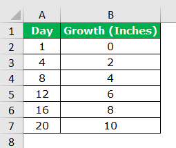
From the above table, a farmer wants to know how tall the paddy was on the 5th day.

By looking at the data, we can easily estimate that on the 5th-day, the paddy was at 2.5 inches. We can easily tell the growth of the paddy crop because it has grown in a linear pattern, i.e., there is a relationship between the number of days recorded and the inches paddy has grown. Below is the graph to show the linear growth of the paddy.

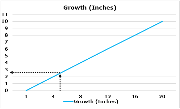
The above graph easily shows the linear growth pattern of the paddy. But if the paddy has grown in a linear pattern, it is tough to predict the 5th-day growth.

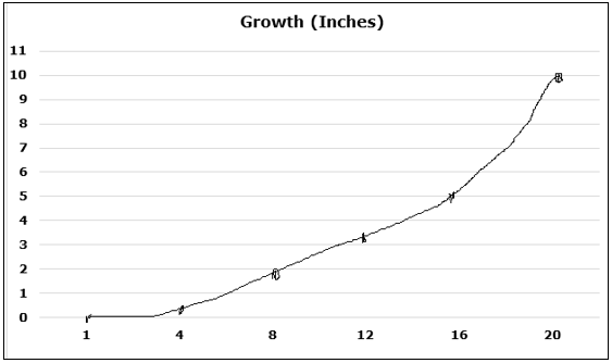
Based on the above curve, farmers cannot estimate what the 5th-day growth was. So, this is where our Interpolation concept helps us find the development on the 5th day.

For interpolation, we have the below formula.

Here, we have two variables, i.e., X1 & Y1. “X” is the first set of values, and “Y” is the second set of values.

In our example of paddy growth, the first set of values is (4,2). So here, “4” is the day, and “2” is the growth inches of the paddy.

The second set of values is (8,4). Here, “8” is the day, and “4” is the growth inches of the paddy.

Since we need to find the growth on the 5th-day variable, “x” becomes 5 to the growth inches variable “y.”

So, let us apply the values to the above formula.

Now, do the first step calculation.

Note “x” is equal to

So, on the 5th-day, paddy growth would be at 2.5 inches.

Example #2

The same Linear interpolation in excel takes the same data to excel.

We need to find the growth inches for the 5th day, so x = 5.

Set 1 (x1, y1)

Set 2 (x2, y2)

So x1 = 4, y1 = 2, x2 = 8, and y2 = 4.

Enter these values in Excel sheet cells.

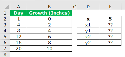
We have mentioned question marks for x1, y1, x2, and y2. Because with this simple data, we can easily find it by just seeing them. But it is always a good practice to find these values through the formula. For example, apply the formula below to find the “x1” value.

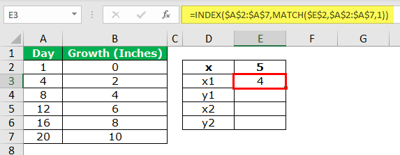
Now, to find the “y1” value apply the below formula.

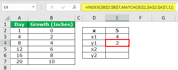
To find the “x2” value apply the below formula.

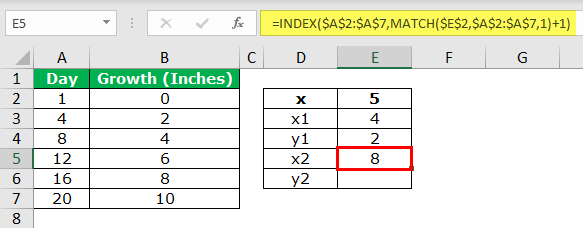
To find the “y2” value apply the below formula.

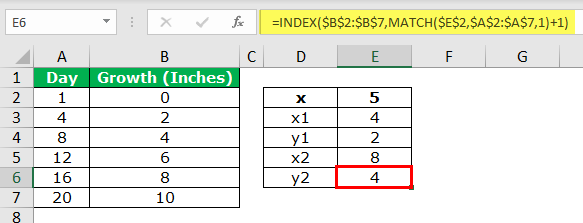
We can find the values for all the Interpolation parameters in the Excel formula.

Next, to find the 5th-day paddy growth inches apply the below formula.

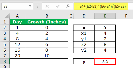
So, as we have calculated manually with the formula, also we got 2.5 as the answer. If needed, we can insert the line graph for the data.

Example #3

Consider the below example showing profit obtained by a company in various months.

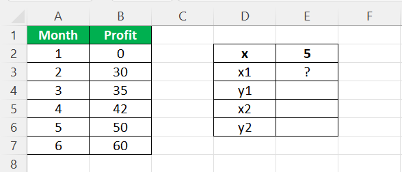
We need to find the profit for the 5th day, so x = 5.

Set 1 (x1, y1)

Set 2 (x2, y2)

So x1 = 4, y1 = 2, x2 = 8, and y2 = 4.

Enter these values in Excel sheet cells.

Now, let us enter the formula, =INDEX($A$2:$A$7,MATCH($E$2,$A$2:$A$7,1)) in cell E3 to find value of x1.

Finally, press Enter key. We can see the result as shown in the below image.

Similarly, we can find the result for other values, y1, x2, y2 with simple formulas.

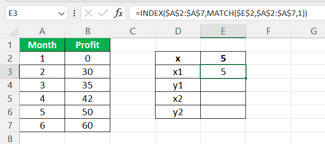
Likewise, we can find the result using interpolation in Excel.

• Interpolation is the process of finding the middle value of the existing data.
• There is no built-in formula in excel to calculate the Excel interpolation value.
• In the MATCH function, we must use “1” for the parameter “match type,” which helps users find the value greater than the lookup value.

This article is a guide to Interpolation in Excel. We discuss how to do data interpolation in Excel and examples and a downloadable Excel template. You may also look at these useful functions in Excel: -

• Get PDF Data into Excel
• Top Examples of Venn Diagram
• Multicollinearity Examples
• Formula of Multiple Regression