How to Group Rows in Excel?

In Excel, organizing the large data by combining the subcategory data is called "grouping of rows." When the number of items in line is not important, we can choose group rows that are not important but only see the subtotal of those rows. On the other hand, when the data rows are huge, scrolling down and reading the report may lead to a wrong understanding, so the grouping of rows helps us hide the unwanted numbers of rows.

The number of rows is also lengthy when the worksheet contains detailed information or data. However, report readers of the data do not want to see long rows. Instead, they want to see a clear view, but at the same time, if they require any other detailed information, they need just a button to expand or collapse them as needed.

This article will show you how to group rows in Excel with expand/collapse to maximize the report viewing technique.

For example, look at the below data.

We have city and state-related sales and cost data in the table above. Still, when we look at the first two rows of the data, we have "California" state and the city is "Los Angeles," but sales happened on different dates. Hence, as a report reader, everyone prefers to read the state-wise sales and city-wise sales in a single column, so we can create a single line summary view by grouping the rows.

Follow the below steps to group rows in excel.

1. First, we must create a subtotal like the one below.

   
   

2. We must select the first state rows (California state), excluding subtotals.

   
   

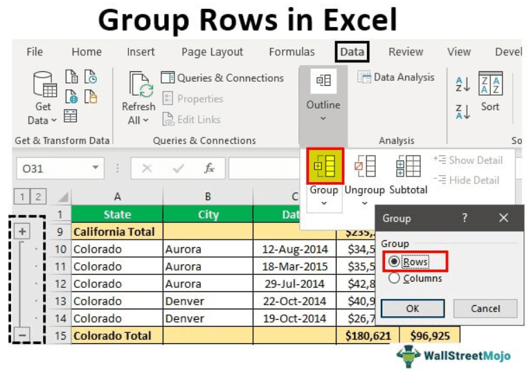
3. Then, go to the Data tab and choose the “Group” option.

   
   

4. Click on the drop-down list in excel of “Group” and choose “Group” again.

   
   

5. Now, it may ask whether to group rows or columns. Since we are grouping Rows, we must choose Rows and click on OK.

   
   

6. The moment we click on OK, we can see a joint line on the left-hand side.

   
   

7. Then, we must click on the minus icon and see the magic.

   
   
   Now, we can see the total summary for the city California. Again, if we want to see a detailed overview of the city, we can click on the plus icon to expand the view.

8. Now again, select the city Colorado and click on the Group option.

   
   

9. As a result, it will group for the Colorado state.

   
   

Group by Using Shortcut Key

With a simple shortcut in excel, we can easily group selected rows or columns. The shortcut key to group the data is "SHIFT + ALT + Right Arrow key."

First, we must select the rows that need to be grouped.

To group these rows, we must press the shortcut key "SHIFT + ALT + Right Arrow key."

In the above, we have seen how to group the data and row with expanding and collapse options using the "PLUS" and "MINUS" icons.

The only problem with the above method is that we need to do this for each state individually, so this takes a lot of time when there are many states. So, what would be your reaction if we say you can group with just one click?

Amazing. Using the "Auto Outline," we can automatically group the data.

Example #1 - Using Auto Outline

First we need to create subtotal rows.

Now, we must place a cursor inside the data range. Under the "Group" drop-down, we can see one more option other than "Group," which is "Auto Outline."

The moment we click on this "Auto Outline" option, it will group all the rows above the subtotal row.

How cool is this??? Very cool, isn’t it??

Example #2 - Using Subtotals

If grouping the rows for the individual city is the one problem, then even before grouping rows, there is another problem: adding subtotal rows.

When there are hundreds of states, it is a tough task to create a subtotal row for each state separately, so we can use the "Subtotal" option to create a subtotal for the selected column quickly.

For example, we had the data like the below before creating the subtotal.

Under the "Data" tab, we have an option called "Subtotal" right next to the "Group" option.

Click on this option by selecting any of the cells of the data range. It will show the below option first up.

First, select the column that needs a subtotal. In this example, we need subtotal for "State," so choose the same from the drop-down list of "At each change in."

Next, we need to select the function type since we add all the values to choose “Sum” function in excel.

Now, select the columns that need to be summed. We need the summary of the "Sales"and "Cost" columns, so choose the same. Click on "OK."

We will have subtotal rows shortly.

Did you notice one special thing from the above image???

It has automatically grouped rows for us!!!!

• The shortcut key for grouping rows is the "Shift + ALT + Right Arrow" key.
• We should sort subtotal that needs data.
• The "Auto Outline" option can group all the rows above the subtotal row.