Homoscedasticity

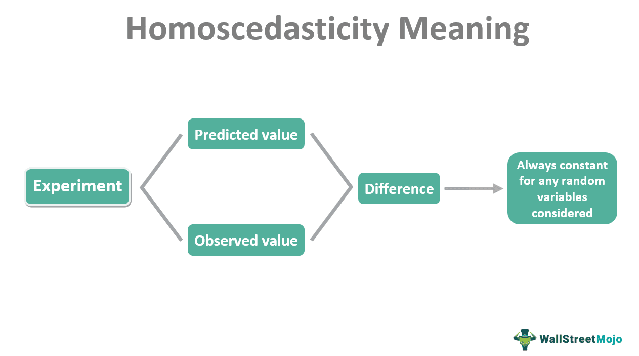
Homoscedasticity refers to the difference between predicted and observed values of an experiment being constant for any random variables considered. It is an important assumption based on which many statistical tests can be conducted. Homoscedasticity test results are considered more reliable owing to unbiased estimates.

Homoscedasticity analysis is a significant concept used and understood widely in econometrics. Its application in statistical programs and tests offers important insights and inferences that can be of high economic value. Moreover, it is also useful in machine learning algorithms and statistical pattern recognition.

• Homoscedasticity can be referred to as the condition of homogeneity of variance. This is because the variance between the predicted and observed values will be a constant for any independent variable.
• Many statistical tests require such an assumption as the basis to get less biased results. Thus, homoscedasticity is a significant concept in econometrics.
• Heteroscedasticity is the opposite phenomenon, whereby the difference between the predicted and observed values will be different, thus increasing the degree of scatter.

Homoscedasticity refers to functions that depend on random events or experiments. For example, in regression, there are usually dependent and independent variables. The value of the dependent variable will keep changing with the independent variable. For example, the time taken for an ice cube to melt depends on the temperature. Here, the temperature is the independent variable, and the time is the dependent one.

So, what is regression analysis? Regression in statistics is used to understand the relationship between multiple variables. The simplest regression analysis will have one independent variable (predictor) and one dependent variable (outcome). Therefore, by changing the values of the independent variable, it is possible to arrive at the different values of the dependent variable. When plotted on a graph, these values will give the regression line.

It is also possible to calculate the expected value from the regression line. However, when experimenting, it is not always necessary that the observed value corresponds to the predicted value. So, in practicality, one can always expect a difference in the expected and actual value. This difference is known as the residual. But in a single regression line, there are many points where one can find the expected and corresponding actual values. A collection of all these residual points is what determines homoscedasticity.

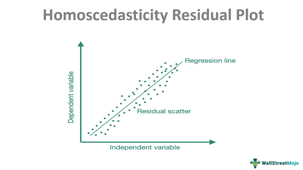
Let us refer to the homoscedasticity residual plot given below. It is a plot of different values of the dependent variable against varying values of the independent variable.

According to the assumption of homoscedasticity, the residuals would be constant. Thus, the degree of scatter will be less. The residuals plotted on the graph, corresponding to each predicted value, will form a region of the slim area around the regression line.

Many homoscedasticity tests use this assumption. Therefore, the difference between the predicted and the observed values is considered a constant, and the tests are done. This provides stability and unbiased results. Also, additional predictor variables are usually considered if there is a lack of homoscedasticity.

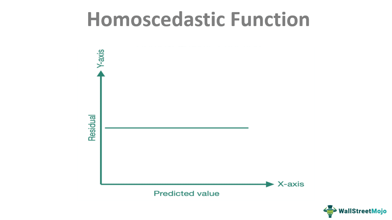
The graph of homoscedasticity is plotted with the predicted value of the dependent variable corresponding to the independent variable taken along the X-axis. The residuals correlate to each predicted value given along the Y-axis.

As can be seen from the graph, the curve is a straight line parallel to the X-axis. This line shows that there might be variations between the predicted and the residual value. Still, this variation should be constant, as should be the case, following the assumption of homoscedasticity.

Now, the zero-slope line is a theoretical inference. Experiments will indicate that the difference between the predicted value and residuals will not always be the same, but the degree of difference should be less.

Suppose a graph was plotted with the predicted value along the X-axis and the observed value along the Y-axis. The curve would be a straight line that would pass through the origin when extended. It would indicate that the observed value should be directly proportional to the predicted value. However, this, too, is an ideal situation, and the line might not be exactly straight.

Nevertheless, the graph should not be confused with the homoscedasticity residual plot. Instead, this is the theoretical mathematical representation of the concept.

Consider the example of students in a class who wrote an exam. Suppose the teacher wants to understand the relation between a student’s IQ and the marks obtained. So the teacher plots the graph by taking IQ as the independent variable and the marks obtained as the dependent variable.

The teacher would expect a straight line passing through the origin because marks should correlate to IQ. However, the observed values might be different. Consequently, the residual or error wouldn’t be constant. This can be because IQ is not the only determinant of marks. Factors like hard work, mental state at the exam time, etc., affect the marks too. Thus, the model is not homoscedastic.

Scedastic functions refer to conditional variance, which is the variance of a particular random variable corresponding to another variable. That is, provided a certain condition, to what degree a function varies. Scedasticity is of two types – homoscedasticity and heteroscedasticity.

If the variance is somewhat the same, the function will be homoscedastic. Therefore, the degree of scatter will be less. In such a case, estimates of the standard error (deviation from the mean) tend to be unbiased. As a result, the overall test results will be promising.

On the contrary, if the observed values appear irregularly from the regression line, the degree of scattering increases, leading to a difference in variances. Hence, there will be no easily recognizable pattern, and the values will appear random. This can lead to a bias in standard error estimation, thus contributing to less reliable test results.

This article has been a guide to Homoscedasticity and its meaning. We explain its assumption, graph, example, and comparison with heteroscedasticity. You may also find some useful articles here -

• Linear Regression
• Two-Way ANOVA
• T-Test