HLOOKUP in Excel

The HLOOKUP function of Excel looks for the specified value in the topmost row of the table and returns another value from the same column of a different row. The specified value is called the lookup value and the value returned is known as a match. This match corresponds with either the exact lookup value (exact match) or with a value close to the lookup value (approximate match).

For example, cells A1 and B1 contain 10 and 20 respectively. Cells A2 and B2 contain “a” and “b” (without the double quotation marks) respectively. The formula “=HLOOKUP(10,A1:B2,2,0)” returns “a,” as shown in the following image.

The given HLOOKUP formula can be interpreted as follows:

• 10–HLOOKUP searches for this value.
• A1:B2–HLOOKUP searches in the topmost row of this array.
• 2–HLOOKUP returns a value from this row of the array.
• 0–HLOOKUP returns an exact match.

HLOOKUP stands for horizontal lookup in excel. It looks up values horizontally (in rows), unlike vertical lookup (VLOOKUP), which looks up values vertically (in columns). Therefore, one must use the HLOOKUP when there is a need to search across (from left to right) in the topmost row of the array.

The purpose of using the HLOOKUP excel function is to quickly retrieve data based on certain predefined parameters. This function is categorized under the Lookup and Reference functions of Excel.

The syntax of the HLOOKUP function in excel is shown in the following image:

The HLOOKUP excel function accepts the following arguments:

• Lookup_value: This is the value to be searched. It can be a numeric value, text string or cell reference.
• Table_array: This consists of two or more rows where the lookup value is to be searched. It can be a range, table or named range. The lookup value must always be located in the topmost row of the “table_array.” Further, this topmost row can contain numeric values, text strings or logical values (true and false).
• Row_index_num: This is the exact row of the table array from which the match is to be returned. For instance, if the “row_index_num” is 3, a value from the third row of the table array is returned.
• Range_lookup: This can take either of the two logical values, which are described as follows:
  • True (1): If the “range_lookup” is true or 1, the HLOOKUP returns an approximate match. Moreover, when this argument is set at true and an exact match is not found (refer to the succeeding note), the function returns the next largest value, which is less than the lookup value. If the “range_lookup” is true, the values of the table array must be sorted in an ascending order, beginning from left to right.
  • False (0): If the “range_lookup” is false or 0, the HLOOKUP returns an exact match. Moreover, when this argument is set at false and an exact match is not found, the function returns the “#N/A” error. If the “range_lookup” is false, no sorting of the table array is required.

The arguments “lookup_value,” “table_array,” and “row_index_num” are mandatory, while the “range_lookup” is an optional argument. If the “range_lookup” argument is omitted, the HLOOKUP excel function assumes it as 1 (true).

Note: When the “range_lookup” argument is set at true, the HLOOKUP function searches for an exact match at first. If the exact match is not found, an approximate match is returned by the function. When the “range_lookup” argument is set at false, the HLOOKUP function searches for an exact match only.

Let us consider some examples to understand the working of the HLOOKUP function of Excel.

Example #1–Exact Match to Retrieve Numerical Values Including a Date

The following image shows the sales revenue (row 6) generated and the profits (row 5) earned on particular dates (row 7) by an organization. This organization operates in four regions, namely, East, West, North, and South. The data for every region is shared. One column represents the data of one region.

We want to retrieve the profit, sales revenue, and the date of sales associated with the Northern region. Use the HLOOKUP function of Excel to perform a lookup with an exact match.

The steps to retrieve the data related to the Northern region are listed as follows:

Step 1: Enter the following formulas in cells B10, C10, and D10 respectively:

1. “=HLOOKUP($A10,$A$4:$E$7,2,0)”
2. “=HLOOKUP($A10,$A$4:$E$7,3,0)”
3. “=HLOOKUP($A10,$A$4:$E$7,4,0)”

Cell A10 contains “north.”

Step 2: Press the “Enter” key after entering each formula in the preceding step. The outputs are shown in cells B10, C10, and D10 of the following image.

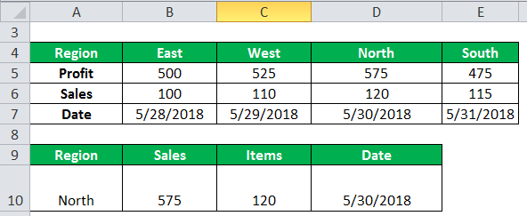
Explanation: In all the three formulas (entered in step 1), the HLOOKUP looks for the value in cell A10, which is “north.” This value is looked up in the topmost row of the array A4:E7. Since the “range_lookup” is 0 in all three formulas, the HLOOKUP excel function looks for an exact match.

In pointer “a” (of step 1), the HLOOKUP returns a value from row 2 of the table array. The column from which the match is returned is the same as that of the North region (column D). The value which corresponds with the stated row and column is 575. Hence, from the formula in pointer “a,” the output is 575. This is the profit of the Northern region.

Likewise, in pointers “b” and “c” (of step 1), the HLOOKUP returns a value from rows 3 and 4 of the table array (A4:E7) respectively. In both formulas, the value is returned from the column North (column D).

So, the corresponding matches for pointers “b” and “c” are 120 and 5/30/2018 respectively. The former match is the sales revenue generated, while the latter is the date of sales related to the Northern region.

Example #2–Exact and Approximate Match to Retrieve Percentages

The following image shows certain random dates (row 15) and percentages (row 16). We want to retrieve the following values:

• The percentage of 1-Jan by performing a lookup with an exact match
• The percentage of 2-Apr by performing a lookup with an approximate match

Use the HLOOKUP function of Excel. Note that all dates pertain to the year 2011.

The steps to retrieve the given values are listed as follows:

Step 1: Enter the following formulas in cells B20 and B21 respectively:

1. “=HLOOKUP(A20,A15:E16,2,0)” or “=HLOOKUP(A20,A15:E16,2,False)”
2. “=HLOOKUP(A21,A15:E16,2,1)” or “=HLOOKUP(A20,A15:E16,2,True)”

Cells A20 and A21 contain “1-Jan” and “2-Apr” respectively.

Step 2: Press the “Enter” key after entering the preceding formulas. The outputs in cells B20 and B21 are 10.0% and 20.0% respectively. These are shown in the following image.

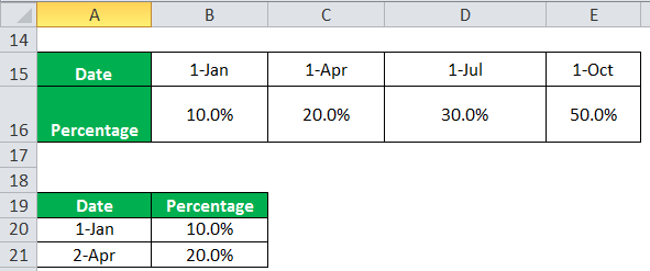
Explanation: In the formula of pointer “a” (entered in step 1), the HLOOKUP excel function looks for the value of cell A20 in the topmost row of the given table array (A15:E16). It looks for an exact match of the lookup value (1-Jan). This exact match is returned from the second row of the table array.

The column from which the exact match is returned is the same as that of 1-Jan (column B). Therefore, the corresponding value at the given row and column is 10.0%, which is the output of the first formula.

Likewise, in pointer “b” (of step 1), the HLOOKUP function searches for the value of cell A21, which is 2-Apr. This is also searched in the topmost row of the array A15:E16. However, this time the function looks for an approximate match as the “range_lookup” argument is set at 1 (or true).

The HLOOKUP excel function is unable to find an exact match of the lookup value (2-Apr) in the topmost row of the table array. So, the function returns the percentage corresponding to the next largest date, which is 1-Apr. This next largest date (1-Apr) is smaller than the lookup value (2-Apr).

Since the match needs to be from the second row of the given array (A15:E16), the output is 20.0%.

Note: The dates in cells B20 and B21 pertain to the same year (2011) as those given in the dataset. Had we entered the dates with different years, we would not have been able to retrieve the required data.

The errors returned by the HLOOKUP excel function are explained as follows:

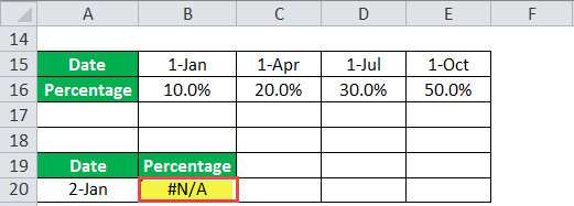
a. “#N/A” error: This is returned if the “range_lookup” argument is set at false (or 0) and the HLOOKUP is unable to find the lookup value in the topmost row of the table array.

For instance, in the following image, the “lookup_value” is 2-Jan and an exact match is required. In cell B20, the formula “=HLOOKUP(A20,A15:E16,2,0)” returns the “#N/A” error.

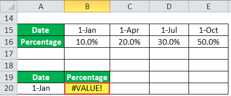
b. “#VALUE!” error: #VALUE! error is returned if the “row_index_num” entered is less than 1.

For instance, in the following image, the “row_index_num” is supplied as zero. In cell B20, the formula “=HLOOKUP(A20,A15:E16,0,0)” returns the “#VALUE!” error.

c. “#REF!” error: This is returned if the “row_index_num” entered is greater than the total rows of the table array.

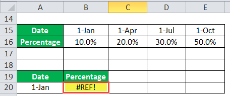
For instance, in the following image, the “row_index_num” is supplied as 3, while the total rows of the “table_array” are 2. In cell B20, the formula “=HLOOKUP(A20,A15:E16,3,0)” returns the “#REF!” error.

The key points related to the HLOOKUP excel function are listed as follows:

• It is a case-insensitive function. This implies that the uppercase and lowercase values are treated the same.
• It is unable to look up anywhere else other than the topmost row of the table array. So, the lookup value should always be located in this row.
• It supports the usage of the wildcard characters like the asterisk (*) and question mark (?) in the “lookup_value” argument. In such cases, one can enter an incomplete text string as the “lookup_value” and, based on this, retrieve the corresponding value.
• It returns the first match in case there is more than one instance of the lookup value in the topmost row of the table array. To avoid such a situation, remove the duplicates before applying the HLOOKUP formula.

Note: If the lookup value is not located in the topmost row of the table array, a combination of the INDEX and MATCH functions can be used to fetch data.