Table Of Contents
How to Hide Formulas in Excel?
Hiding formulas in Excel is a method when we do not want them to be displayed in the formula bar when we click on a cell with formulas. We can format the cells, check the hidden checkbox, and then protect the worksheet. It will prevent the formula from displaying in the "Formula" tab. Only the result of the formula will be visible.
13 Easy Steps to Hide Formula in Excel (with Example)
Let us understand the steps to hide formulas in Excel with examples.
Step 1:
Following are the 13 steps that we can use to hide formulas in Excel:
- First, we must select the entire worksheet by pressing the shortcut key "Ctrl + A."

- Now, on any cell, right-click and select "Format Cells" or press "Ctrl + 1."

- Once the above option is selected, it may open the below dialog box and select "Protection."

- Once the "Protection" tab is selected, uncheck the "Locked" option.

As a result, this will unlock all the cells in the worksheet. Remember, this may unlock the cells in the active worksheet in all the remaining worksheets. It remains locked only. - If we observe as soon as we unlock the cells, Excel will notify us of an error as "Unprotected Formula."

- Select only the formula cells and lock them. For example, we have three formulas in the worksheet, and we selected all three.

- Now, we must open the "Format Cells, select the "Protection" tab, and check the "Locked" and "Hidden" options.

Note: If we have many formulas in the Excel worksheet, we want to select each one of them, then we need to follow the below steps. - Now, press the F5 (shortcut key to "Go to Special") and select "Special."

- Consequently, this will open up the below dialog box. Select "Formulas" and click "OK." It would select all the formula cells in the worksheet.

Now, it has selected all the formula cells in the entire worksheet. - Protect the sheet once the formula cells are selected, locked, and hidden. Then, go to the "Review" tab and "Protect Sheet."

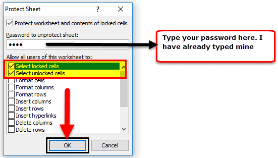
- Click on the "Protect Sheet" in Excel, and the dialog box may open up. Select only "Select locked cells" and "Select unlocked cells." Type the password carefully because we cannot edit those cells if we forget the password.

- Click on the "OK" button. It will again ask us to confirm the password. Enter the same password again.

- Click on the "OK." Now, our Excel formulas are locked and protected with a password. Suppose we cannot edit the password without the password. Then, if we try editing the formula, Excel will show the below warning message for us. Also, the formula bar does not show anything.

Things to Remember
- The most common way of hiding the formulas is by locking the particular cell and password protecting the worksheet.
- The first basic thing we need to do is "unlock all the cells in the active worksheet." You must be wondering why we need to unlock all the cells in the worksheet where we did not even start the process of locking the cells in the worksheet.
- We need to unlock first by default. Then, Excel turns on excel Locked cell. However, we can still edit and manipulate the cells because we have not yet password-protected the sheet.
- We can open the "Go to Special" dialog box by pressing the "F5" shortcut.
- We must use the "Ctrl + 1" as the shortcut key to open the formatting options.
- Remember the password carefully. Otherwise, we cannot unprotect the worksheet.
- Only the password known person can edit the formulas.

