Group Columns in Excel

Group Column in Excel means bringing one or more columns together in an Excel worksheet. It enables an option to contract or expand the column, and Excel provides us a button to do so. To group columns, we must select two or more columns, and then from the "Data" tab in the "Outline" section, we have the option to group the columns.

Example #1

Example #2

• Step 1: We must first select columns B and C.

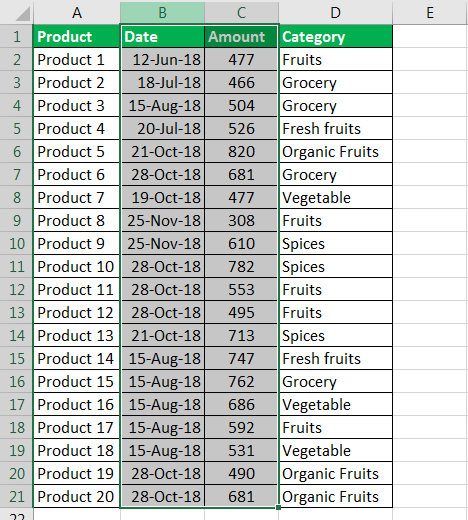
• Step 2: Go to the "Data" option in the excel toolbar and select the "Group" option in the outline toolbar, as shown below.

• Step 3: Next, go to the option group and make the group of a column selected.

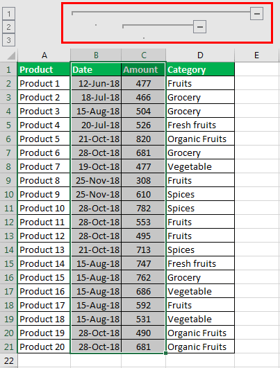
Now, we can see the two minus signs; two groups are created in a particular spreadsheet that we want to group.

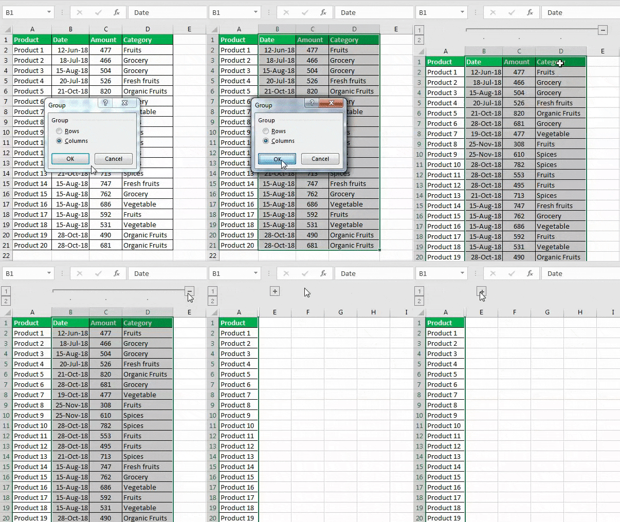
• Step 1: First, We must click on the created minus sign while grouping the column.

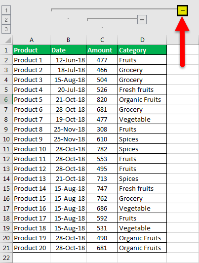
• Step 2: When we click on the minus sign, a column will collapse, resulting in the hide in a column.

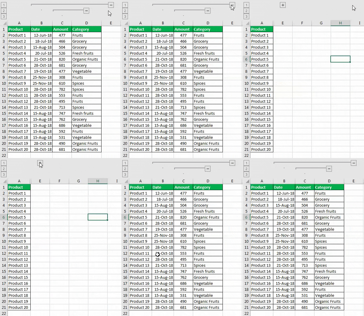
• Step 3: Once we click on the minus sign, it automatically shows the plus sign, which means that if we want to unhide the column, click on the plus sign to unhide the columns.
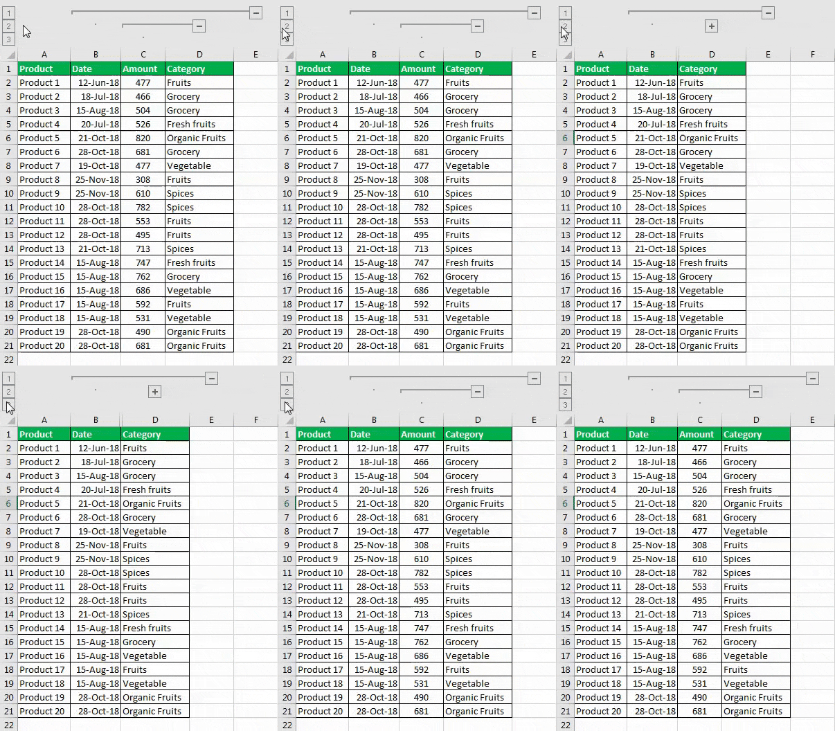
• Step 4: We can likewise utilize the small numbers in the upper left corner. They let us cover up and unhide all groupings of a similar dimension without a moment's delay. For instance, in the table on the screen capture, clicking on 2 will conceal columns B and D. This is particularly helpful if we made a progressive collection system. Likewise, clicking on 3 will unhide or hide columns C and D.

• Step 1: First, we must select the data. Then, press the Shortcut Excel Keys – Shift + Alt + right arrow. We may see the dialog box in the Excel spreadsheet as follows:

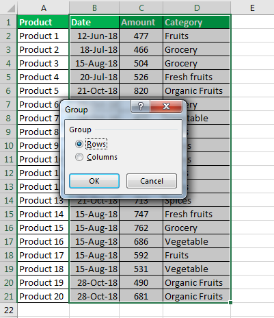
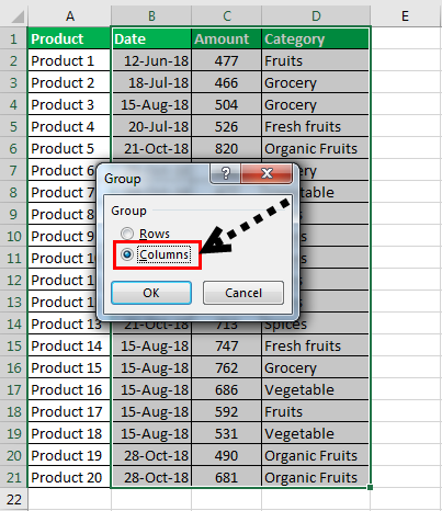
• Step 2: Select the radio button on a column to hide the columns in excel.

• Step 3: Click on the "OK." Now, we can hide and unhide the columns in excel.

1. To effectively expand and contract the section or areas of a worksheet.
2. To limit schedules or side estimations that different users probably would not require while working in Excel worksheets.
3. To keep data composed and in an organized structure.
4. To make new sheets (tabs) as a substitute.
5.  It is a better option than hiding cells.
6. It is a better function as compared to hiding the column function.
7. It helps to set up the grouping level.

1. We would not be able to make a group of cells that are not adjacent.
2. If we manage different worksheets and need to assemble similar lines/columns on numerous worksheets in the meantime, it is impossible to use this function.
3. We always need to check that the data is in a sorted form.
4. We always need to check while grouping the column in Excel to select the correct column that needs to group.

1. We would not be able to add the calculated items to grouped fields in the Excel spreadsheet.
2. It is impractical to choose a few non-nearby columns.
3. Clicking on the minus icon may hide the column, and the icon may change to the plus sign letting us instantly unhide the data.
4. We can select the range and press "Shift + Alt + left arrow" to remove the grouping from the Excel spreadsheet.