Table Of Contents
What Is The Go To Special Excel?
The Go To Special Excel option helps find and select cells containing a specific category of data and those satisfying the required criterion.
Users can use the Go To Special function to choose blank cells or cells containing constants, formulas, or objects. Also, while the option enables users to select cells based on row and column differences, the option helps highlight the precedent and dependent cells in a sheet.
For example, the following dataset lists the US states and their capitals.
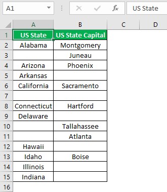
The task is to find and select the blank cells in the source dataset. Then, we can use the Go To Special Excel Blanks option to achieve the required output.
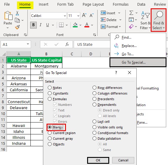
In the above Go To Special Excel Blanks example, we select a cell in the active sheet and choose the Go To Special option function under the Find & Select option in the Home tab.
Clicking the menu Go To Special Excel option opens the Go To Special window, where we must select the Blanks option and click OK.
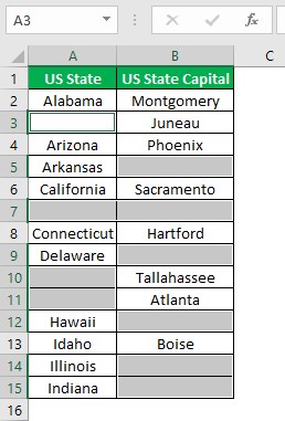
The above step will highlight the blanks in the source dataset, with the first empty cell being the active cell.
Table of contents
- The Go To Special Excel function enables one to identify and select cells meeting the specified criterion or containing a specific data type.
- Users can use the Go To Special option to find and highlight empty cells or cells containing constants, objects, formulas, and comments. The function also helps locate and select precedents and dependents based on one active cell, visible cells, and conditionally formatted cells.
- We can apply the Go To Special function using the option under the Find & Select option in the Home tab. Otherwise, we can use the keyboard shortcut Alt + H + FD + S.
How To Use Go To Special Excel?
We can use the menu Go To Special Excel option or the keyboard shortcuts to open the Go To Special window and access the listed options.
The steps to use the Go To Special function from the ribbon are as follows:
-
Select the required cell in the active sheet.
-
Choose the Home tab - The Find & Select option down arrow - The Go To Special function.
-
The Go To Special window will open.
-
We can find Go To Special Excel condition from the list in the window based on which we want to choose the cells in the sheet.
-
Once we select the specific criterion, click OK to close the Go To Special window and view the required cells satisfying the selected criterion.
Furthermore, the following Go To Special Excel shortcut options help us access the function quickly:
- Press Alt + H + FD + S to open the Go To Special window.
- Press F5, Ctrl + G, or Alt + H + FD + G to open the Go To window. Next, press Alt + S or select Special in the Go To window to open the Go To Special window.
The first Go To Special Excel shortcut option directly opens the Go To Special window. However, the shortcuts in the second open the Go To window, from where we can access the Go To Special window.
Examples
Check out the following examples explaining how to find Go To Special Excel function and apply the criterion to select the required cells.
Example #1 - Find And Select Row And Column Differences
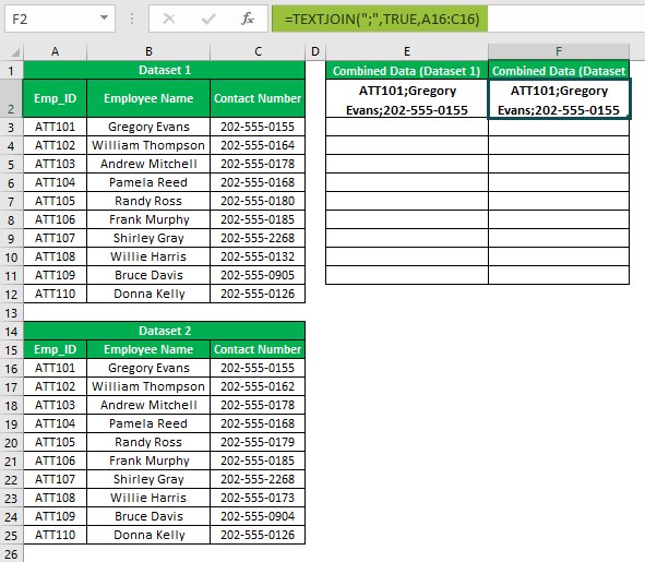
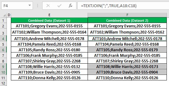
The following image shows two datasets.
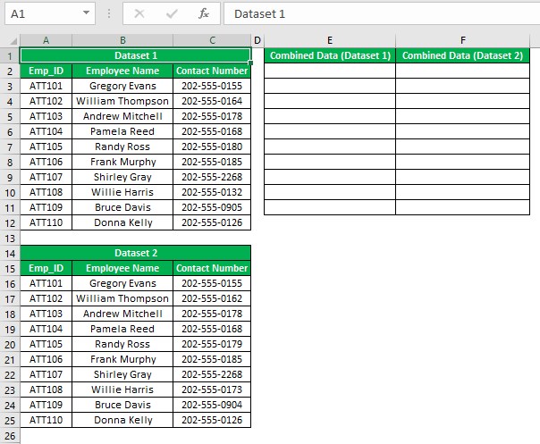
The requirement is to combine the data in the two sets and display the concatenated data in columns E and F.
Furthermore, highlight the cells based on the row differences in the range E2:F11, containing the combined data values.
Then, the steps are as follows:
Step 1: Choose cell E2, enter the Excel TEXTJOIN function, and press Enter.
=TEXTJOIN(";",TRUE,A3:C3)

Next, choose cell F2, enter the TEXTJOIN(), and press Enter.
=TEXTJOIN(";",TRUE,A16:C16)
Step 2: Select cells E2:F2.

Next, use the Excel fill handle to update the formula in the cell range E3:F11.
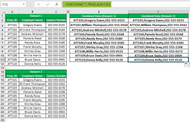
The TEXTJOIN() accepts three inputs. The first argument, delimiter, is Semi-colon and the second argument, ignore_empty, is TRUE, indicating the formula to ignore blank cells. Next, the third argument, text1, is the cell range containing the text values to join.
Thus, the output in the range E2:F11 shows the concatenated data of the two datasets, with a Semi-colon in between.
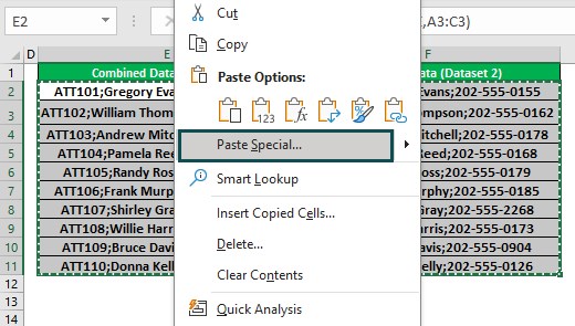
Step 3: Select the cell range E2:F11 and right-click to choose Copy in the contextual menu.

Next, right-click the copied cell range to choose Paste Special from the context menu.
After that, click the Paste Special option right arrow to choose the first option under the Paste Values section.
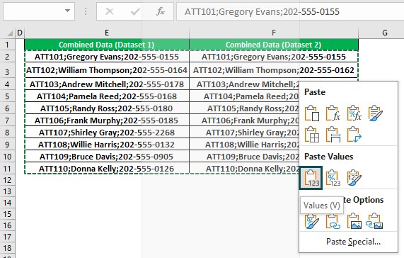
The option will paste the copied data as values in the chosen cells.
Step 4: Select the cell range E2:F11. Next, choose Home - Find & Select - Go To Special or use the keyboard excel shortcut Alt + H + FD + S to open the Go To Special window.

Next, select the Row differences option and click OK in the Go To Special window.

The Row differences option compares the column E and F cells row-wise in the chosen range. It then highlights the column F cells in the rows where the column F cell value differs from the corresponding column E cell value.
Please note that the option checks for row differences in each row in the chosen range individually.
Furthermore, assume we introduce another dataset in the range H1:J11, displaying the employee list from the two source datasets and their assigned tasks.
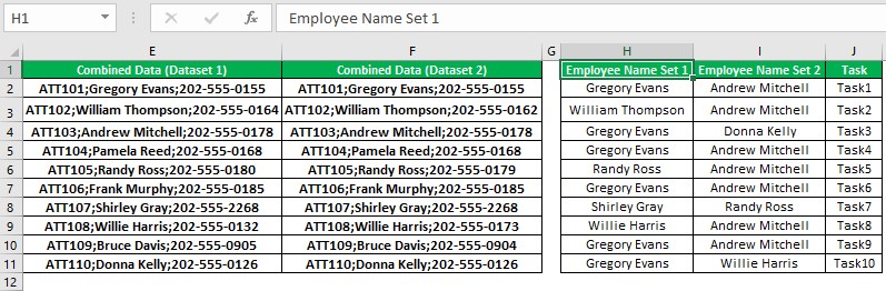
The aim is to highlight the cells based on the column differences in the range H2:I11, containing the two sets of employee names.
Step 5: Choose the range H2:I11 and select Home - Find & Select - Go To Special.

Step 6: The Go To Special window opens, where we must choose the Column differences option.
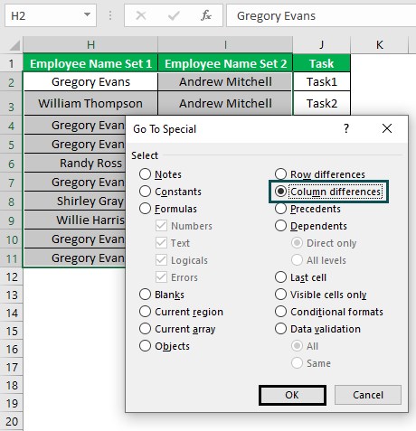
Finally, click OK in the Go To Special window to close it.
By default, the active cell in the chosen range is cell H2. So, the Column differences option will check and highlight the cells in the range H3:H11 that contain data different from that in cell H2.
Likewise, the option checks and highlights the cells in the range I3:I11 that contain data different from that in cell I2. The reason is that the option considers the cells in the row containing the initial active cell as the current cells for the rest of the corresponding columns for comparison.

Again, the Column differences option checks for each column’s differences in the chosen range individually.
Example #2 - Find And Select Precedents And Dependents
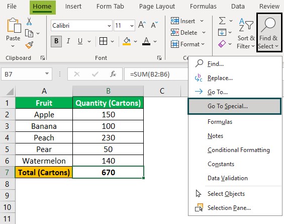
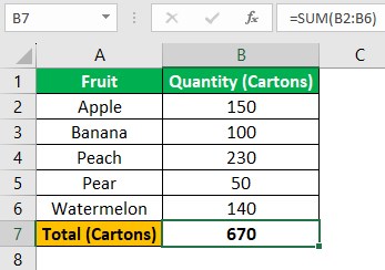
The following dataset contains fruits, their quantities and the total quantity data.
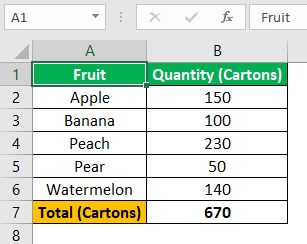
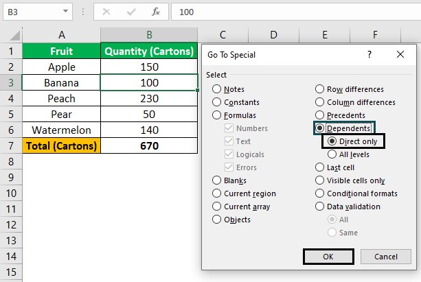
The requirement is to determine the direct precedents of cell B7 and the direct dependents of cell B3 in the active sheet.
Step 1: Choose cell B7 and select Home - Find & Select - Go To Special.
Step 2: The Go To Special window will open, where we must choose the Precedents option.
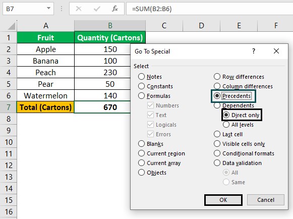
The above action will enable the Direct only and All levels option under the Dependents option. So, we choose the Direct only option to meet our requirements.
Next, click OK to close the window and the direct precedent cells of the active cell B7 get selected in the active sheet.
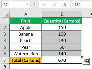
The above output indicates that the active cell B7 formula refers to cells B2:B6.
Step 3: Choose cell B3 and select Home - Find & Select - Go To Special.
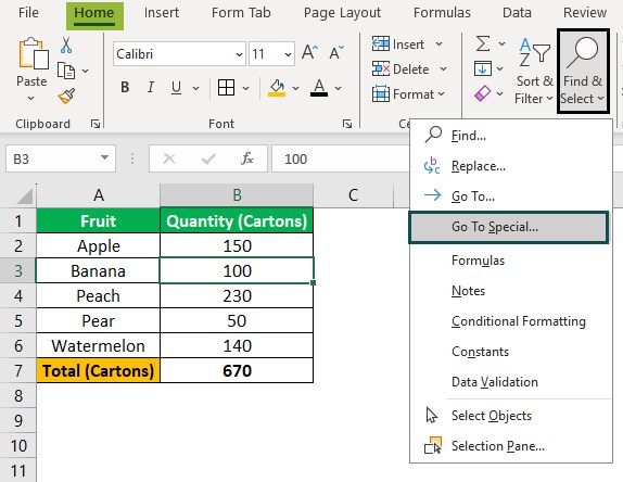
Step 4: The Go To Special window will open, where we must choose the Dependents option.
Furthermore, the above action will enable the Direct only and All levels options under Dependents. We will select the Direct only option to fit our requirements.
Clicking OK in the Go To Special window will close it, and the directly dependent cells of the active cell get selected in the active sheet.
The above output indicates that cell B7 is directly affected by the active cell B3.
Example #3 - Find And Select Constants
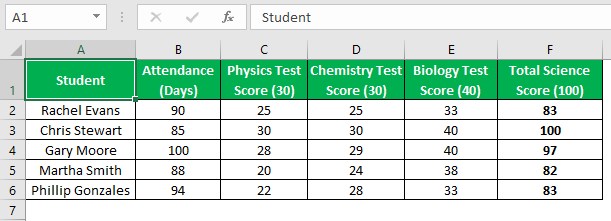
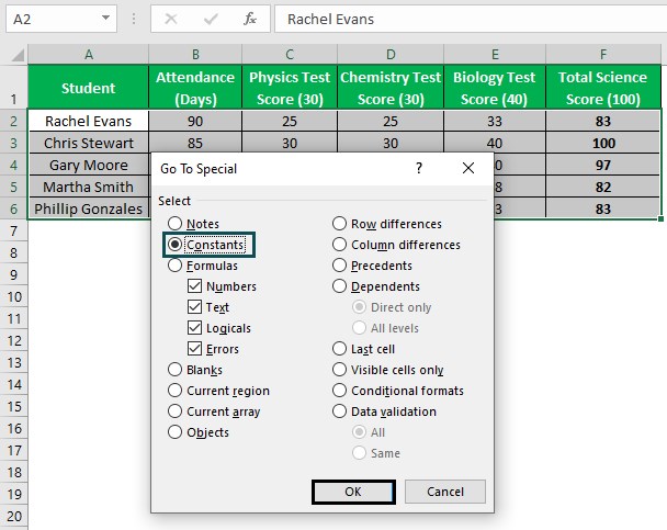
The following dataset lists students, their attendance and the total scores data based on their test scores in three subjects.
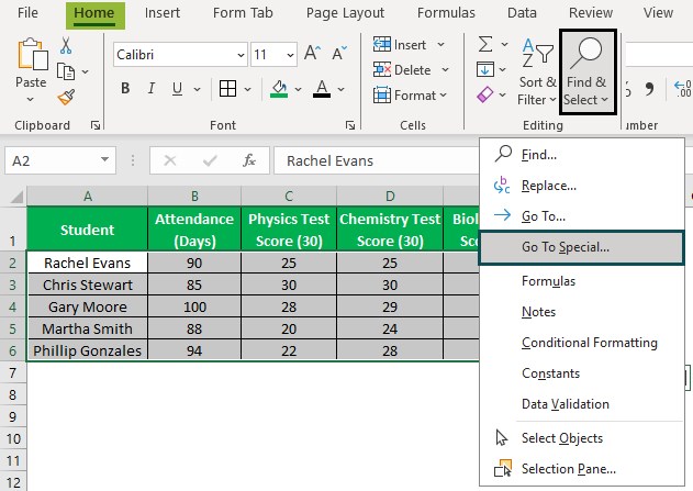
The requirement is to find and select the cells containing constants in the source dataset.
Step 1: Choose the range A2:F6 and select Home - Find & Select - Go To Special.
Step 2: The Go To Special window opens.
Select the Constants option in the Go To Special window.
Clicking OK in the Go To Special window will close it, and the cells containing constants in the chosen range will appear selected in the active sheet.
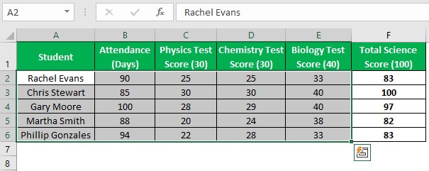
The output shows that cells A2:E6 contain constants and hence appear selected, with the first cell A2 containing a constant value being the active cell.
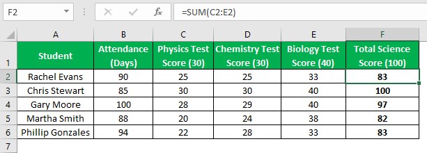
On the other hand, cells F2:F6 appear unselected since they contain formulas instead of constants, as depicted below.
Example #4 - Find And Select Visible Cells
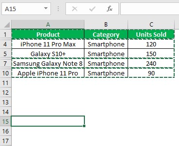
The following dataset lists laptops and smartphones and their units sold data.
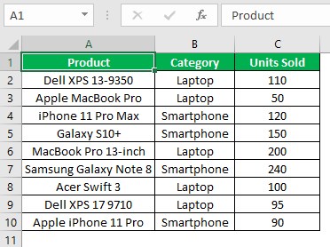
Consider the task to hide the rows containing laptops’ data and then copy and paste the rows containing the smartphones’ data in cell A15.
Step 1: Click the row 2 number to select the entire row. Next, while pressing Ctrl, click on row numbers 3, 6, 8, and 9 to select the rows.
After that, right-click on a chosen row to choose Hide from the context menu.
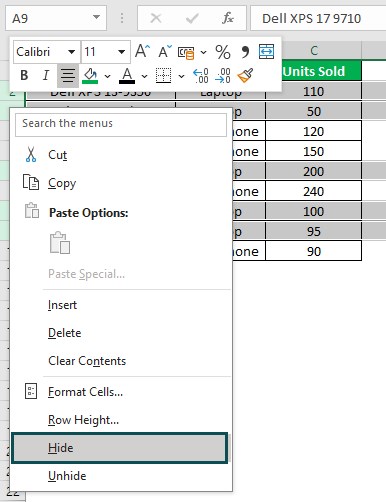
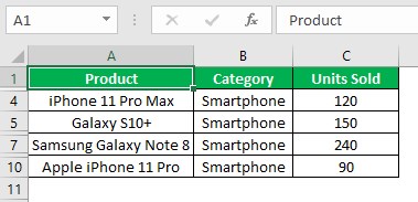
The above step will hide the chosen rows while the remaining rows in the source dataset remain visible.
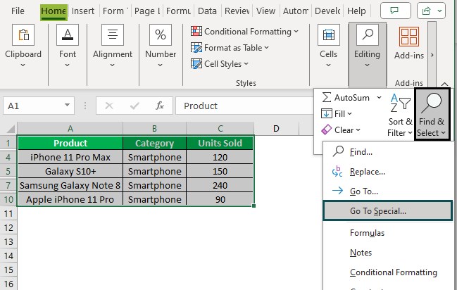
Step 2: Select the source dataset and choose Home - Find & Select - Go To Special.
Step 3: The Go To Special window opens, where we must choose the Visible cells only option.
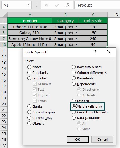
Clicking OK in the Go To Special window will close it, and the visible cells in the chosen cell range will appear selected.

Step 4: Press Ctrl + C to copy the values in the chosen visible cells.

Next, select the target cell A15.
Finally, press Ctrl + V to paste the copied data into the target cell.
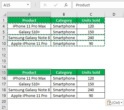
On the other hand, assume we do not use the Visible cells only option. Then, the rows of data hidden in the source dataset would also get pasted in the target cell when we select the source dataset and copy the data.
Important Things To Note
- Ensure the Excel version is not online. Otherwise, the Go To Special Excel option will not be available.
- The Go To Special option highlights the row and column differences in each chosen row and column individually based on the active cell in the corresponding row and column. Also, ensure the specific rows and columns, where we must determine the differences, do not contain formulas. Otherwise, the correct cells will not get highlighted.
Frequently Asked Questions (FAQs)
You can delete blanks in Excel using Go To Special, as explained below with an example.
The following dataset contains a list of branch offices and their sales representatives.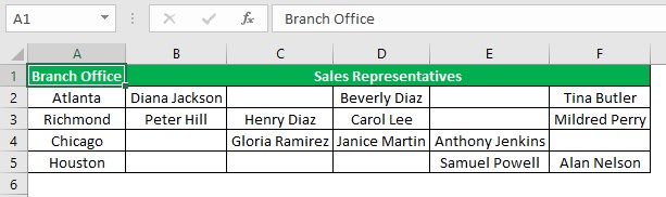
The task is to select the blanks in the range B2:F5 and delete them in the source dataset.
Step 1: Choose the range B2:F5 and then select Home - Find & Select - Go To Special.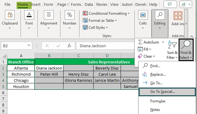
Step 2: The Go To Special window will open, where we must choose the Blanks option.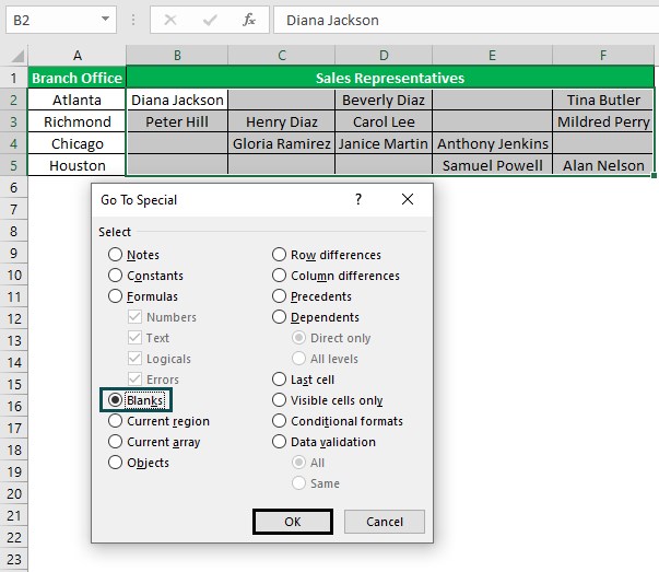
Clicking OK in the Go To Special window will close it, and the blank cells in the chosen cell range will appear selected.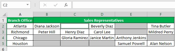
Step 3: Right-click on a chosen cell to select Delete in the context menu.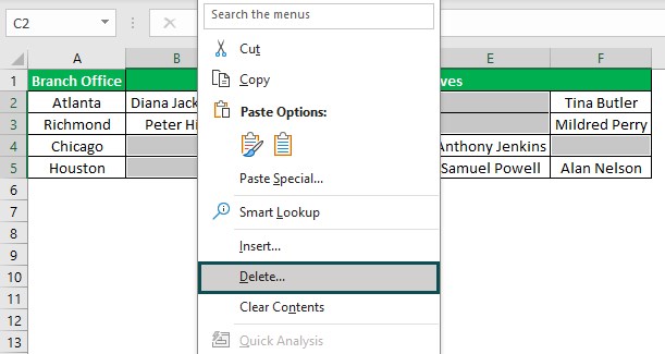
Step 4: The Delete window will open, where we must choose the Shift cells left option.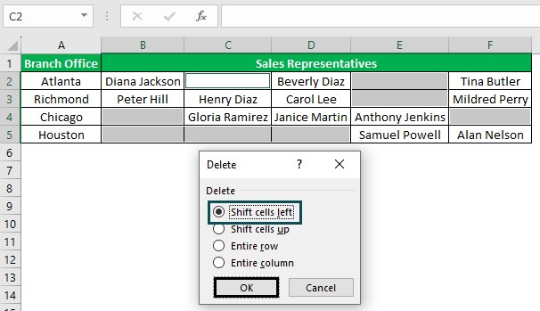
Clicking OK in the Delete window will close it, with the chosen blank cells deleted and the remaining cells shifted to the left.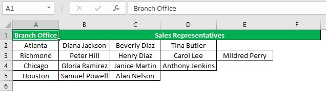
The Go To Special in Excel Mac shortcut key is pressing F5 to open the Go To window and then selecting the Special button or typing the Command-S.
You don’t have Go To Special in Excel because Excel is the online or web version.
Download Template
This article must be helpful to understand the Go To Special Excel, with its formula and examples. You can download the template here to use it instantly.
Recommended Articles
This has been a guide to What Is Go To Special Excel. We explain the different ways to use the Go To Special Excel option with examples & points to remember. You may learn more from the following articles –
