Table Of Contents
GetPivotData Excel Function
The GETPIVOTDATA function in Excel is a query function in Excel that is used to fetch values from a PivotTable based on some specific criteria such as the structure of the PivotTable or the reference provided to the function. This function can only be applied on the PivotTable and not on the normal table arrays.
For example, assume we want to calculate the sum of sales of vegetables for a specific month from the PivotTable. in such a scenario, we can use the GETPIVOTDATA function and get the result.
Formula

Three parameters are used in GETPIVOTDATA.
- Data_field: Name or value that you are looking for.
- Pivot_Table: Any cell reference or range of cells in the pivot table.
- ,,,,etc: Up to 126 pairs of fields and item names can be found. This is an optional part of GETPIVOTDATA.
Note: The values must be present in the below details:
- We can directly insert the number.
- Use the date in the serial number or use the date function in Excel.
How to use the GetPivotData Function in Excel? (Examples)
Example #1
Suppose we have a "Region" in the first column, a "Month" in the second column, "Agent" names in the third column, "Sales" in the fourth column, and a "Target" in the sixth column. Now, we have to find the total sales using the GETPIVOTDATA function. Below is the data. We can copy it and paste it into Excel for practice.

Now, create a PivotTable.

Below is the Image as well for your understanding.

Below is an example of using the GetPivotData function to find out total sales.
=GETPIVOTDATA("Sale",C4)
=GETPIVOTDATA("Sum of Sale",C4)
Example #2
The next question is to find out the total target by using the GETPIVOTDATA function.
(Use the same data mentioned above)
=GETPIVOTDATA("Target",D4)
=GETPIVOTDATA("Sum of Target",D4)
Example #3
In the next question, by using the same data, let us determine the sale of Mar month.

Now, there are two ways to find the sale in March. First, we can type items of field names in the GETPIVOTDATA in the Excel function. In the second one, we can refer to worksheet cells.
=GETPIVOTDATA("Sale",C4,"Month","Mar")
=GETPIVOTDATA("Sale",C4,A4,A9)
Example #4
In the next question, by using the same data, let us determine the "Target of Mar" month.

=GETPIVOTDATA("Target",D4,"Month","Mar")
=GETPIVOTDATA("Target",D4,A4,A9)
Here, we need to know important things.
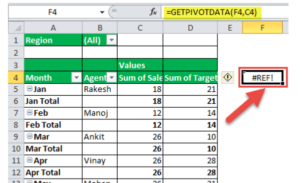
If we change the first argument, data_field, to a reference F4, the result is a GETPIVOTDATA #REF! Error.

So, we must always remember to use text in the data_field syntax to ignore errors.
Example #5
Let us move to another task of using dates in the GETPIVOTDATA function.
If we use dates in the GETPIVOTDATA formula, there might be a few errors. Below are a few examples.
In the below-given table, we have a "Date" in the first column and a "Sale" in the second column.

Now, create a PivotTable.

By using this table, find out the sale of 26th May.
To get a correct answer while typing a date, we must use the following formula:
=GETPIVOTDATA("Sale",B3,"Date","5/26/2018")
Things to Remember
There are two kinds of errors found in the GETPIVOTDATA function.
- The GETPIVOTDATA Excel function will return a #REF! Error if any supplied field name is incorrect.
- The GETPIVOTDATA function always accepts the name of the data_field and field/item values in the double quotes.

