FV Function In Excel

The FV function in Excel is a financial function used to calculate the future value of an investment based on constant periodic payments and a constant interest rate. It helps determine how much an investment will be worth after a number of periods, assuming regular contributions and compounding interest. The function takes several arguments including rate, number of periods, payment, present value, and payment type.

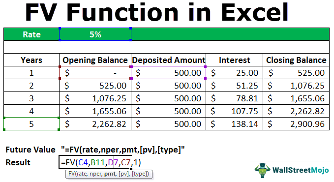
For example, suppose a $2,000 investment is made for 6 years in the savings account with 10% annual simple interest. In this scenario, using the FV function, we can calculate the investment’s future value(fv). In this case, the future value(fv) of the $2,000 investment will be:

For example, if you invest 1000 every month for 5 years at an annual interest rate of 6 percent, compounded monthly, the formula would be 

=FV(0.06/12, 60, -1000). 

This returns approximately $ 69,770. It shows the future value of your regular monthly investment after 5 years, assuming the interest compounds monthly.

The syntax of the FV function in Excel is as follows:

The FV formula in Excel takes up five arguments, as shown above in the syntax. They are:

• rate – It is the rate of the interest per period.
• nper – It is the total number of payment periods in an annuity.
• pmt – It is the payment made each period. It cannot change. Generally, it does not include fees or other taxes but does cover the principal and total interest.
• pv – The present value, or the total amount that a series of future payments is worth now.
• type – is the number 0 or 1 and indicates when payments are due. If the type is omitted, it is assumed to be 0. The 0 types are used when payments are due at the end of the period and 1 at the beginning.

We can use the FV function by knowing details such as the rate, total payments period and the present value. We can enter the function manually and look at it through a simple example. 

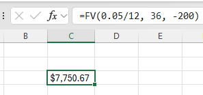
Suppose we wish to know how much we will have in hand after saving $200 every month for 3 years, with an annual interest rate of 5 %, compounded monthly. Let us look at how to use the FV function in Excel to calculate this future value.

Step 1: Let us find the interest rate per period. As the annual rate is 5% and interest is compounded monthly,we enter the first argument as 0.05/12.

Step 2: We will find the total number of periods. Making monthly payments for three years means 3 * 12 = 36.

Step 3: The payment amount per period is $200. We enter this as -200 because it is a cash outflow.

Step 4: Now let us use the FV formula: =FV(0.05/12, 36, -200)

Step 5: Press Enter, we get approximately $7750. This is the amount you will have after 3 years of saving.

FV in Excel is very simple. Let us now see how to use the FV function in Excel with the help of some examples.

As we dive into the complexities of this topic, it becomes clear how foundational knowledge can lead to practical applications. Those interested in enhancing their skills further might find this Investment Banking Mastery Program (IBMP) helpful for gaining deeper insights.

Example #1

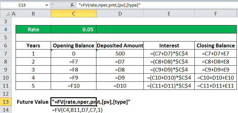
For example, if you deposit an amount of $500.00 for 5 years at the rate of interest provided at 5%, then we will calculate the future value that it will receive at the end of the 5th year in the following manner.

It can be directly calculated using the FV function in Excel. When,

• rate = 5%
• nper = 5 years
• pmt = deposited amount each year ($500.00)
• pv = 0 (at the start of Year 1)
• type = 0 and 1 ( 0 means payment received at the end of the period, 1 payment received at the beginning of the period)

So, according to the FV formula, it will calculate the FV in Excel as:

 =fv(rate,nper,pmt,,)

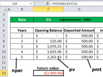
Here, the type is 1 because we receive the payment at the start of each period. 

The fv value calculated using the future value function is within the red parenthesis that denotes the negative value. It is usually negative because, in the end, the bank pays out the amount. Thus, it signifies the outflow and inflow of the amount.

This can be verified by calculating the FV amount manually. 

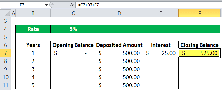
At the beginning of the year (1st year), the opening balance will be nil, $0.

Now, let us assume that the amount deposited in the account is $500.00.

Here,

• Opening Balance = OB
• Deposited Amount = DA
• Rate of Interest = R
• Interest Amount = I
• Closing Balance = CB

So, the interest in 1st year at the 5% will be

 (OB + DA)*R

= (0+500)*0.05 equals to $25.00

So, the closing balance of the 1st year will be

(OB+DA+I)

= (0.00+500.00+25.00) equals to $525.00

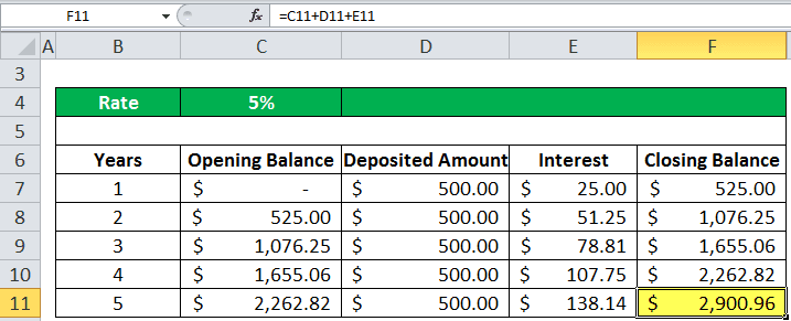
The deposited amount in column D remains the same throughout the 5 years. But, at the end of the 5th year, the value that will have each year will be added with interest. So, let us calculate this manually first, then we will be using the FV Excel function to get the desired result figured out automatically, thus saving time and effort.

In column C, we have the opening balance each year. In the first year, we have to start opening a balance with a nil account; the amount will be 0$.

In column E, we have the interest payment for each year. For example, an interest rate is 5% in cell C1. So, the interest payment in the first year will be the sum of the opening balance and deposited balance times the interest value.

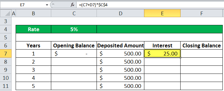
So, in the first year, we received the interest value amount of $25.00. Then, finally, the closing balance in column F will be calculated as the sum of all the balances that the sum of the opening balance, deposited amount, and the interest amount.

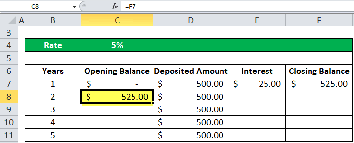
So, $525.00 will be the opening balance for the next year, the second year.

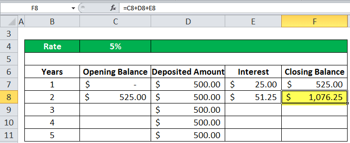
Again, we are receiving a deposit of $500.00 in the second year. Similarly, the interest is calculated in the same manner.

So, at the end of the 5th year, calculating it the same way, we get the final future value amount, which is $2900.96.

Example #2

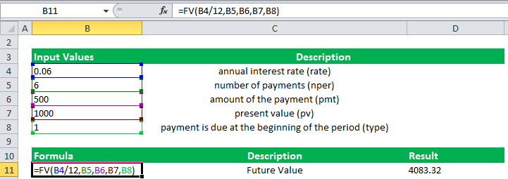
If the annual interest rate is 6%, the number of payments is 6, the payment amount is $500, and the present value is $1,000. Therefore, the payment due at the beginning of the final period will be the future value calculated below in the screenshot.

We enter all the details manually at first as shown below.

Apply the formula in cell B11 as shown.

=FV(0.06/12,6,500,1000,1).

Press Enter. 

1. The nper and rate specified have to be consistent. For example, if payments are monthly on a four-year loan at 10% annual interest, we must use 0.1/12 for rate and 4*12 for nper. If we make annual payments on the same loan, we must use 10% or 0.1 for the rate and 4 for nper.
2. The cash we payout, such as deposits to savings, is represented by negative numbers for all the arguments. But conversely, the cash we receive, such as dividend checks, is represented by positive numbers.