FREQUENCY in Excel

The FREQUENCY function in Excel helps in calculating the frequency of a data value within a given range of values. In other words, it estimates how many times a data value has occurred amongst a given set of values. It provides a vertical array of numbers that correspond to each value's frequency within a range. It is a built-in statistical function of Excel.

The syntax of FREQUENCY function is stated as follows:

The FREQUENCY Formula has the following mandatory arguments:

• Data_array –It is an array or reference to a set of certain values whose frequencies we need to count.
• Bins_array–It is an array or reference to intervals into which you want to group the values in “data_array.”

This function returns an array of values. In Excel, it is used as an array formula using “CTRL+Shift+Enter” (For Mac: Press “Command+Shift+Enter”). Select the cell in which the output is required. Then type the FREQUENCY formula in Excel and enter the array formula.

Select cells --> Type formula --> Press “CTRL+Shift+Enter”

FREQUENCY function in Excel returns a frequency distribution of the “data_array” in the “bins_array” intervals. The output is always one more than the number of elements in “bins_array.” The extra element in the returned array corresponds to the count of values higher than the highest element of the “bins_array.” Suppose the “bins_array” contains three elements {2, 4, 6}, the function will return four elements {<2, 2-4, 4-6, >6}.

If “data_array” contains no values, the FREQUENCY function returns an array of zeros. If “bins_array” contains no values, the FREQUENCY function returns the total number of elements given in “data_array.”

Sometimes, it is required to understand the frequency distribution of a given data rather than the data itself. For example, the age of individuals in a population varies greatly; hence you need to visualize it as frequencies. Similarly, marks obtained by each student in a class need clubbing in terms of frequencies to understand the overall performance of the class.

The function is very simple and easy to use. Let us understand how it works with the help of some examples.

Example #1

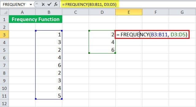
We have numbers {1, 3, 2, 4, 6, 2, 3, 4, 5} in B3:B11 for which the frequency is to be calculated. 

Example #2

A survey was conducted. It collected data related to the height of the participants. The results are given in the following table.

Now, calculate the frequency for the intervals mentioned below.

< 155

155-160

160-165

165-170

> 170

E4:E7 are showing the intervals {155, 160, 165, 170}.

Now, let us do the frequency calculation with the steps mentioned below.

• Start by selecting five cells that are consecutive (4 + 1).

• Enter the below-mentioned formula:

“=FREQUENCY(B4:B14, E4:E7)”

• Press “CTRL+Shift+Enter.”

This returns the frequency of the height for the specified intervals (shown in the subsequent image).

Example #3

A list of IDs of students who have failed in one or more subjects in a class is mentioned below. The table also includes the subjects in which they have failed. Those who have failed in either one subject or more are considered as fail.  Find out the number of students who have failed.

To identify the number of students who have failed, use the following formula:

“=SUM(--(FREQUENCY(B4:B9, B4:B9) >0))”

It returns 4 as the number of failed students (as shown in the subsequent image).

Let us look at the details of the formula.

FREQUENCY(B4:B9, B4:B9) calculates the frequency of data B4:B9 using the interval B4:B9. It returns {1; 1; 2; 0; 2; 0; 0}.

FREQUENCY(B4:B9, B4:B9) >0 checks if the obtained frequency is greater than zero. It returns the logical value “true” if it is greater than zero, else “false.” It returns {TRUE; TRUE; TRUE; FALSE; TRUE; FALSE; FALSE}.

SUM(--(FREQUENCY (..) >0)) will sum up the “true” and return the number of unique values.

Example #4

The data of daily customer visits to a supermarket is shown in the table below. The time of their visit is also given. The data is displayed in cells B4:C39. We want to see at which time intervals the customers visited the most in the store. This will help us plan the employees’ working hours efficiently. The store opens at 11:00 a.m. and closes at 8:00 p.m.

Let us first decide on the time interval. We use the following intervals for the sake of simplicity:

• 11:00 a.m.
• 12:00 a.m.
• 1:00 p.m.
• 2:00 p.m.
• 3:00 p.m.
• 4:00 p.m.
• 5:00 p.m.
• 6:00 p.m.
• 7:00 p.m.
• 8:00 p.m.

• Select the cells G4:G13 in the table, where the frequency is obtained.  The store closes at 8:00 p.m. Hence, we need not select the cell for >8:00 p.m., as it is zero in all the cases.

• Now, enter the following formula:

“=FREQUENCY(B4:C39,G4:G13)”

• Press  “CTRL+Shift+Enter.” 

It returns the frequency of customer visits to the store. In this case, we observe the maximum customer visits between 5:00 p.m. – 6:00 p.m.

• The FREQUENCY function in Excel gives the frequency distribution of the given data (“data_array”) into the given intervals (“bins_array”).
• The FREQUENCY formula in Excel is entered as an array formula. 
• To calculate frequency, a range of adjacent cells is selected into which the distribution is required to appear. 
• To enter the FREQUENCY formula in Excel, press “CTRL+Shift+Enter” (for Mac, press “Command+Shift+Enter”).
• For “x” number of elements in the “bins_array,” select “x + 1” number of cells, while entering the FREQUENCY formula in Excel. The extra cell returns the number of values in “data_array,” which is greater than the third interval value. 
• The FREQUENCY formula ignores blank cells and text.

This has been a guide to the FREQUENCY Function in Excel. Here, we discuss how to use this function along with step by step examples and downloadable template. You may also look at these useful functions in Excel –

• VBA Select Cell
• How to use INT Formula?
• COS Excel Function
• MEDIAN in Excel