Table Of Contents

Freeze Panes in Excel

Last Updated :

Blog Author :

Edited by :

Reviewed by :

Example #1–Freeze the Top Row in Excel

The following image shows the sales revenue (in $ in column B) generated in various countries (column C) by the different sales personnel (column A) of an organization. The entire data relates to the four quarters of a year.

We want to freeze the top row (row 1) of the given dataset.

Freeze the top row Example 1

The steps for freezing the first row in Excel are listed as follows:

Click the "freeze panes" drop-down from the "window" group of the View tab. Select "freeze top row" as shown in the following image.
The entire first row (row 1) is frozen. A horizontal gray line appears right below row 1. This line indicates that the row immediately above is frozen.
To cross-check, one can scroll down the worksheet. The row containing the column headers is fixed. The same is shown in the following image.

Example #2–Freeze the First Column in Excel

Working on the data of example #1, we want to freeze the first column (column A) of the given dataset.

The steps for freezing the first column of Excel are listed as follows:

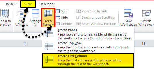
Step 1: From the “window” group of the View tab, click the “freeze panes” drop-down. Select “freeze first column,” as shown in the following image.

Step 2: The entire first column (column A) is frozen. A vertical gray line appears right next to column A (or between columns A and B). This line indicates that the column immediately to the left is frozen.

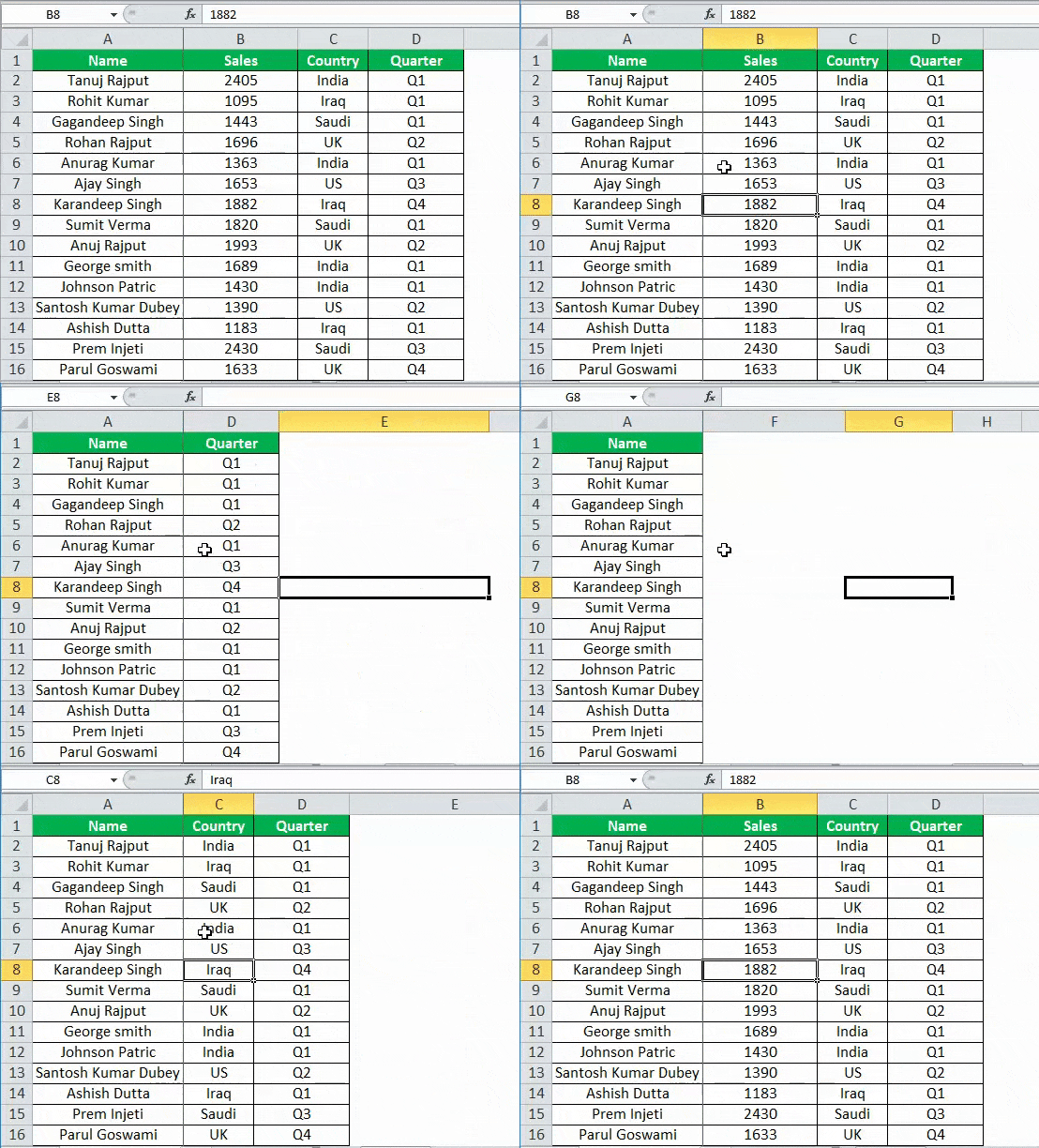
If one scrolls from left to right, column A stays at its place. The same is shown in the following image.

Example #3–Freeze the Top Row and the First Column Together

Working on the data of example #1, we want to freeze the first row (row 1) and the first column (column A) simultaneously.

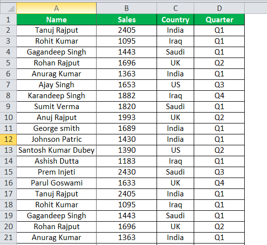
The steps to freeze the first row and the first column simultaneously are listed as follows:

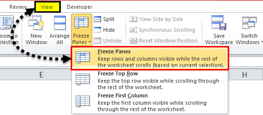
Step 1: Select the cell B2. From the “freeze panes” drop-down (in the View tab), select “freeze panes.” The same is shown in the following image.

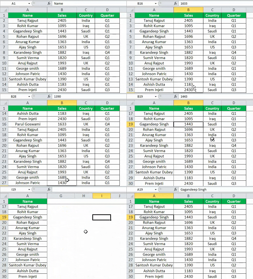
Step 2: Row 1 and column A, both are frozen. A horizontal grey line appears below row 1 and a vertical grey line appears right next to column A. The same is shown in the following image.

The row immediately preceding the active cell (B2) is frozen. Likewise, the column immediately to the left of cell B2 is also frozen.

Note: One must select the cell (in step 1) cautiously. This is because the “freeze panes” option works on the basis of the current selection. It freezes the rows and columns immediately preceding the active or the selected cell.

Freeze Multiple Rows and Columns Together in Excel

The steps to freeze multiple rows and columns are listed as follows:

Step 1: Select the correct cell. The selected cell should be positioned as follows:

a. The selected cell should be immediately below the last row to be frozen.
b. The selected cell should be to the immediate right of the last column to be frozen.

Follow both the pointers a and b to freeze multiple rows and columns simultaneously.

Step 2: Select “freeze panes” from the “freeze panes” drop-down of the View tab.

The rows and columns immediately preceding the selected cell (selected in step 1) are frozen.

Note: It is also possible to freeze either multiple rows or multiple columns. One can freeze as many rows and/or columns as one wants. However, the freezing of multiple rows and/or columns should begin from the first row (row 1) and the first column (column A) respectively.

Shortcut to Freeze Panes in Excel

The shortcuts to freeze panes in excel are mentioned as follows:

To freeze rows and columns both: Press the keys “Alt+W+F+F” one by one. This freezes rows and columns preceding the currently selected cell.
To freeze the top row only: Press the keys “Alt+W+F+R” one by one. This freezes the first row (row 1) of the worksheet irrespective of the currently selected cell.
To freeze the leftmost column only: Press the keys “Alt+W+F+C” one by one. This freezes the first column (column A) of the worksheet irrespective of the currently selected cell.

Unfreeze Panes in Excel

The steps to unfreeze panes in excel are listed as follows:

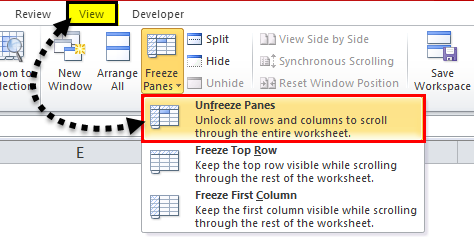
Step 1: Click the drop-down arrow of “freeze panes” in the “window” group of the View tab.

Step 2: Click “unfreeze panes,” as shown in the succeeding image. The gray lines, which appeared as a result of freezing, will disappear.

The “unfreeze panes” option is quite useful when one is unable to figure out where the freezes have been applied in the worksheet.

Note 1: The “unfreeze panes” option appears (under the drop-down of “freeze panes”) after one or more rows and/or columns are frozen by the user.

Note 2: Once the “unfreeze panes” option is clicked, the rows and columns are no longer fixed. So, the worksheet prior to freezing is displayed.

The Purpose of Freezing Panes in Excel

The objectives of freezing panes in excel are listed as follows:

To prevent referring to the same set of data repeatedly, thus saving the scrolling time of the user
To know which row or column represents which data
To facilitate comparisons of the different sections of the worksheet

Frequently Asked Questions

1. What does freezing panes mean and where is this option in Excel?

Freezing panes helps lock or fix certain rows and/or columns of a worksheet so that they remain stationary with a movement through the database. For instance, while working with large datasets, the user may need to keep the row or column headers visible at all times.

By freezing panes, the scrolling time of the user is reduced. This is because the need to refer to the same worksheet area repeatedly is eliminated. Moreover, making comparisons between the different rows or columns becomes easier.

The "freeze panes" option is available under the "freeze panes" drop-down (in the "window" group) of the View tab of Excel. This option freezes one or more rows and/or columns based on the current selection.

In addition, one can use the options "freeze top row" and "freeze first column" (under the "freeze panes" drop-down) to freeze the first row and the first column respectively.

2. How to freeze panes horizontally and vertically in Excel?

To freeze panes horizontally, the user needs to freeze one or more rows. To freeze panes vertically, one or more columns need to be frozen.

The steps to freeze one or more rows and/or columns are listed as follows:

a. Select the relevant cell. This cell should be immediately below the last row to be frozen. Further, it should be to the right of the last column to be frozen.
b. From the "freeze panes" drop-down (in the "window"d group) of the View tab, select "freeze panes".

The row preceding the active cell (selected in step a) is frozen. Moreover, the column to the left of this cell is also frozen. The gray lines appear which indicate the frozen panes.

Note: With this method, one can freeze any number of rows and columns. The condition is that the freezing of panes must begin from the first row (row 1) and the first column (column A). In other words, the rows and columns in the middle of the worksheet cannot be frozen.

3. How to freeze multiple panes in Excel?

It is possible to freeze multiple rows and columns simultaneously in Excel. However, one cannot freeze panes in the middle of the worksheet. For instance, one cannot create a horizontal pane consisting of rows 9, 10, and 11.

The user can create a horizontal pane which consists of stationary rows beginning from row 1. Likewise, a vertical pane consisting of stationary columns, beginning from column A, can be created.

Apart from one horizontal pane and one vertical pane, it is not possible to create additional panes in the middle of the worksheet. Hence, one cannot create multiple horizontal or multiple vertical panes in Excel.

In other words, a horizontal pane (rows 1, 2, and 3) followed by a scrollable area (rows 4, 5, and 6), and again a horizontal pane (rows 7, 8, and 9) cannot be created.