Formatting in Excel

Last Updated :

Blog Author :

Edited by :

Reviewed by :

Table Of Contents

Formatting in Excel (2016, 2013 & 2010 and Others)

Formatting in Excel is a neat trick used to change the appearance of the data represented in the worksheet. We can do formatting in multiple ways, such as we can format the font of the cells or format the table by using the "Styles" and "Format" tabs available in the "Home" tab.

Formatting in Excel (2016, 2013 & 2010 and Others)

How to Format Data in Excel? (Step by Step)

Let us understand the working of data formatting in Excel by simple examples. Now, suppose we have a simple report of sales for an organization as below:

This report is not attractive to viewers. Therefore, we need to format the data.

Now, to format data in Excel, we must do the following:

Bold the text of the column header.
Make the font size larger.
Adjust the column width using the shortcut key (Alt+H+O+I) after selecting the whole table (Ctrl+A).
Align the data in the center.
Apply the outline border by using (Alt+H+B+T)
Apply background color using the "Fill Color" command available in the "Font" group on the "Home" tab

We will be applying the same format for the table's last "Total" row by using the "Format Painter" command available in the "Clipboard" group on the "Home" tab.

As the amount collected is a currency, we should format the same as "Currency" using the command available in the "Number" group placed on the "Home" tab.

After selecting the cells we need to format as currency, we need to open the "Format Cells" dialog box by clicking the above arrow.

Choose "Currency" and click on "OK."

Data Formatting (currency english india)

We can also apply the outline border to the table.

We will be creating the label for the report by using "Shapes." To make the shape above the table, we need to add two new rows. So, we will select the row by "Shift+Spacebar" and then insert two rows by pressing "Ctrl+’+" twice.

We must choose an appropriate shape from the "Shapes" command available in the "Illustration" group in the "Insert" tab to insert the shape.

Create the shape according to the requirement and with the same color as the heads of the column. Then, add the text on the shape by right-clicking on the shapes and choosing "Edit Text."

We can also use the "Format" contextual tab for formatting the shape using various commands such as "Shape Outline," "Shape Fill," "Text Fill," "Text Outline," etc. We can also apply the excel formatting on text using the commands available in the "Font" group placed on the "Home" tab.

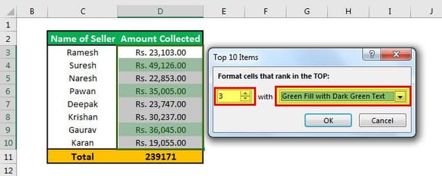
We can also use "Conditional Formatting" to take the viewers' attention to the "Top 3" salesperson and "Bottom 3" salesperson.

Data Formatting (conditional formatting - Top bottom Rules)

Format the cells that rank in the "Top 3" with "Green Fill with Dark Green Text."

Also, format the cells that rank in the "Bottom 3" with "Light Red with Dark Red Text."

Data Formatting (Format Cells - bottom rule)

We can also apply another conditional formatting option, "Data Bars."

Data Formatting (conditional formatting - data bars)

We can also create a chart to display the data, part of "Data Formatting Excel."

Shortcut Keys to Format Data in Excel

To make the text bold: Ctrl+B or Ctrl+2
To make the text italic: Ctrl+I or Ctrl+3
To make the text underline: Ctrl+U or Ctrl+4
To make the font size of the text larger: Alt+H, FG
To make the font size of the text smaller: Alt+H, FK
To open the ''Font'' dialog box: Alt+H,FN
To open the ''Alignment'' dialog box: Alt+H, FA
To center align cell contents: Alt+H, A, then C
To add borders: Alt+H, B
To open the ''Format Cells'' dialog box: Ctrl+1
To apply or remove strikethrough data formatting Excel: Ctrl+5
To apply an outline border to the selected cells: Ctrl+Shift+Ampersand(&)
To apply the "Percentage" format with no decimal places: Ctrl+Shift+Percent (%)
To add a non-adjacent cell or range to a selection of cells using the arrow keys: Shift+F8

Things to Remember

While data formatting in Excel, we must make the title stand out, good and bold, it ensures it conveys the content we are showing. Next, we should enlarge the column and row heads and put them in a second color. Readers may quickly scan the column and row headings to get a sense of how the information on the worksheet is organized. This way, it can help them view what is most important on the page and where they should begin.