Format Numbers To Millions & Thousands in Excel

Publication Date :

08 Mar, 2019

Blog Author :

Edited by :

Reviewed by :

Download FREE Format Numbers To Millions & Thousands Excel Template and Follow Along!

Million Format Excel Template.xlsx

Table Of Contents

What Is Format Numbers To Millions & Thousands In Excel?

Excel number formatting is a larger topic than we think. We have already published the topic Excel Custom Number Formatting, including number formatting in Excel. In today’s article, we will concentrate on million formats of numbers in Excel to allow them to be shown in a shorter form to read and understand very easily.

In the Mathematics field, every number has different terminologies.

For example, one thousand (1,000) is represented as 1k, and one lakh (100,000) is described as 100k.

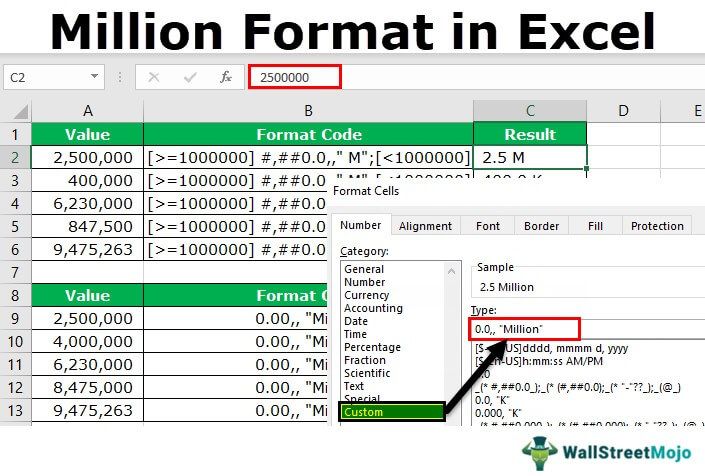
Format-Numbers-To-Millions-Thousands-in-Excel — *You are free to use this image on your website, templates, etc..* *Please provide us with an attribution link*

Similarly, in Excel, we can also format the numbers to show as thousands, “K,” “Millions,” and “Billions.” In this article, we will show you the techniques of modifying or changing the format of the numbers in Excel.

Key Takeaways

Format numbers to millions and thousands in Excel is a technique used to convert numbers into Thousands and Millions.
This method in Excel uses codes to convert numerals into text, i.e., thousands and millions.
Meanwhile, format numbers to millions and thousands in Excel helps users simplify data as long numerals might be difficult to read and process.
For instance, reading 60,000 might be difficult. We can easily convert this value as 60 Thousand using formatting numbers to thousands in Excel method.

How To Do Excel Numbers Formatting – Thousands And Millions?

Let us learn how to format Excel numbers to thousands and millions with simple examples and detailed steps.

#1 – Excel Format Numbers In Thousands & In K’s

Firstly, we will see how to format numbers in thousands and K’s. Remember, both thousand and K are the same but need different formatting techniques in excel.

Assume we have the below set of numbers in the Excel sheet.

Value	Format Code	Result
2,500		??
25,000		??
250,000		??
70,000		??
825,000		??

Now, we need to format these numbers in thousands. So, for example, we do not want to see the number 2500, but instead, we want the formatting as 2.5 Thousand.

To change the view of the numbers, we need to change the formatting of the numbers.

Follow the below steps to change the formatting of the numbers.

We must right-click on the numbers we want to format and select “Format Cells.”

Note: We can also press the “Ctrl + 1” shortcut key to open the “Format Cells.”
Now, we must go to the “Custom” option.
In the “Type:” section, we need to apply the formatting code. Below is the formatting code to change the formatting of the numbers.
Format Code: 0, “Thousands”
Now, we must see values in “Thousands.”

One of the problems here is that 2500 shows as 3 Thousand, but we need the exact value to be viewed here. To make sure decimal values are not rounded up to the nearest thousand, we need to change our formatting code as below.

Format Code: 0.00, "Thousands"

Now, we can see the exact values with decimal points.

#2 – Unconventional Way Of Showing Thousand Values

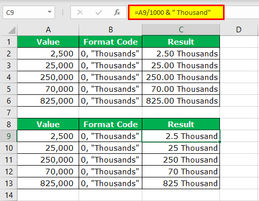
Step #1 – This unconventional method shows a thousand values. The thing we need to do here is, we need to divide the number by 1,000 and combine the word “Thousand” by using the ampersand (&) symbol.

Step #2 - Format numbers in K’s values.

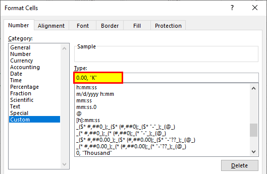
To show a thousand numbers in K’s, we need to change the word “Thousand” to “K.”

Format Code: 0.00, “K”

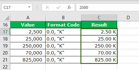
Step #3 - The result is as follows:

#3 – Format Numbers In Millions

In the previous step, we have seen how to format numbers in thousands. Now, we will see how to format numbers in millions.

Step #1 - The previous formatting code would show “10 lakhs” as “1000 K,” “25 lakhs” as “2500 K,” etc.

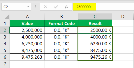
We all know 10 lakh is equal to 1 million. So, we need to format the number in millions instead of in thousands. Below is the code to format the number in millions.

Step #2 - Format Code: 0.00,, "Million"

Only the difference between the previous code and this code is that we have added one extra comma (,). Then we combined the word “Million.”

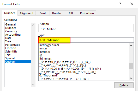
Step #3 - This code would show the result of numbers in “Millions.”

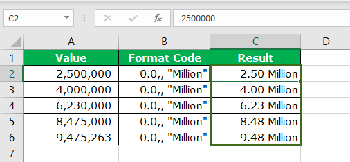
This format code applies only to millions. Imagine we have numbers that are less than 10 lakhs.

For example, 2.5 lakh would be shown as “0.25 Million” instead of “2500 K.” This is the common problem with a single referencing format code.

However, we can modify the code to show the result based on the cell value of numbers. For example, if the value is less than 10 lakh, the result should be K’s. If the value is greater than 1000,000, the result should be “Million.”

Step #4 - Format Code: #,##0.0,,” M”; #,##0.0,” K”;General

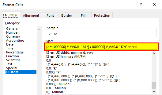
Step #5 - This code will format the numbers according to the number value and show the results accordingly.

Important Things To Note

Instead of “Million,” we can show the alphabet M.
Instead of “Thousand,” we can show the alphabet “K.” These two are alphabetical representations of “Million” and “Thousands.”
To show the negative numbers in red, we must apply the below code.

$#,##0.0,,”M”; $#,##0.0,”K”;General