Excel Format Cells

Formatting cells in Excel is one of the key options used to format the data. We can format data in different formats, such as time, date, currency, font, etc.,

For example, using format cells in excel, we can format time. If the value is 1800 hrs and we want to format it based on hh:mm AM/PM format, we can use the format cells option. As soon as we click format, the 1800 hrs will be formatted into 06:00 PM.

Formatting cells in excel is really simple. Let us have a look at the following examples to learn how to use format cells in excel.

Example #1 - Format Date Cell

Excel stores date and time as serial numbers. We need to apply an appropriate format to the cell to see the date and time correctly.

For example, look at the below data.

It looks like a serial number to us, but we get date values when applying date format in excel to these serial numbers.

The date has a wide variety of formats. Below is a list of formats we can apply to dates.

We can apply any formatting codes to see the date, as shown above in the respective format.

• To apply the date format, we must first select the range of cells and press Ctrl + 1 to open the format window. Then, under Custom, we must apply the code as we want to see the date.

Format Cells Shortcut Key

We get the following result.

Example #2 - Format Time Cell

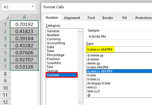
As we said, the date and time are stored as serial numbers in Excel. Now, it is time to see the TIME formatting in excel. For example, look at the numbers below.

The TIME values are varied from 0 to less than 0.99999, so let us apply the time format to see the time. Below are the time format codes we can generally use:

“h:mm:ss”

To apply the time format, we must follow the same steps:

So, we get the following result.

So, the number "0.70192" equals the time of 16:50:46.

If we do not want to see the time in the 24-hour format, we need to apply the time formatting code like the one below.

Now, we will get the result as shown in the below image.

Now, our time is shown as 04:50:46 PM instead of 16:50:46.

Example #3 - Format Date And Time Together

The date and time are together in Excel. We can format both the date and time together in Excel. For example, look at the below data.

Let us apply the date and time format to these cells to see the results. The formatting code is dd-mmm-yyyy hh:mm:ss AM/PM.

We get the following result.

Let us analyze this briefly now.

The first value we had was 43689.6675 for this, we have applied the date and time format as dd-mm-yyyy hh:mm:ss AM/PM, so the result is 12-Aug-2019 04:01:12 PM.

43689 represents data in this number, and the decimal value 0.6675021991 represents time.

Example #4 - Positive And Negative Values

When dealing with numbers, positive and negative values are part of it. To differentiate between these two values by showing them with different colors is the general rule everybody follows. For example, look at the below data.

To apply a number format to these numbers and show negative red values, below is the code.

“#,###;-#,###”

If we apply this formatting code, we can see the above numbers.

Similarly, showing negative numbers in brackets is also in practice. For example, to show the negative numbers in the bracket and red color, below is the code.

“#,###;(-#,###)”

We get the following result.

Example #5 - Add Suffix Words To Numbers

If we want to add suffix words along with numbers and still be able to do calculations, it is great.

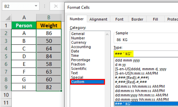
If we show a person’s weight, adding the suffix word KG will add more value to the numbers. Below is the person’s weight in KG.

To show this data with the suffix word KG, apply the below formatting code.

### " KG"

After applying the code, the weight column looks like as shown below.

Example #6 - Using Format Painter

Format Painter Excel, we can apply one cell format to another. For example, look at the below image.

The date format is DD-MM-YYYY, and the remaining cells are not formatted for the first cell. But, we can apply the format of the first cell to the remaining cells by using a format painter.

We must select the first cell, then go to the Home tab and click on Format Painter.

Now, we must click on the next cell to apply the formatting.

Now again, select the cell and apply the formatting, but this is not the smart way of using a format painter. Instead, double-click on Format Painter by selecting the cell. Once we double-click, we can apply the format to any number of cells, applying all at once.

• The format option is used to format the data in different formats.
• We can format the date and time together.
• The Excel Format Painter is the tool used to copy one cell format to another.