Flow Chart In Excel

The flow chart in Excel is also known as a process chart in Excel. It represents different steps involved in a process from start to end. It has predefined shapes to represent every step involved in the process. We need to use the predefined SmartArt templates in Excel to use this chart.

In this article, let us learn how to create flow charts in Excel using different methods in Excel with step by step instructions.

Flow charts in Excel help us show the relationship between two data. So, in turn, it can help people understand the data efficiently.

We need to follow a few steps to create the flow chart in Excel. They are:

• Create a Grid
• Snap to Grid
• Page Layout

Let us learn how to create flow chart in Excel.

We need to follow a few steps to create the flow chart in Excel. They are:

• Create a Grid

We need to adjust the size of the gridlines in excel to make the shapes uniform in size. Then, the Excel worksheet would look like graph paper, so it becomes easy to draw the shapes.

• We need to select all the cells by clicking on the triangle icon at the beginning of the column/row numbers. Keep the cursor on any column headers. Then, right-click and select the “Column Width” option in excel.

• When the "Column Width" screen pops up, we must adjust the number to 2.14 (2.14 equals 20 pixels assuming that the default font is "Calibri" and font size is "11" in Excel) and click "OK."

• Snap to Grid

We can use this option available in Excel to snap the shape to the size of the grid. By enabling this option, whenever we insert the shape into the sheet, it will adjust the shape's size to that of the height and width of the grid.

• Under the "Page Layout" tab in the ribbon, in the "Arrange" section, click on the drop-down below the "Align" option. Then, select the "Snap to Grid" option in the drop-down option.

• Page Layout

We should adjust the page layout of the sheet by setting the page break, margins, and orientations if we want to take the printout of the flow chart or we want to copy it to other applications like Word because it would be difficult to set the layout once the Excel flow chart is built.

We can set the page's orientation as either "Portrait" or "Landscape" based on the flow of the diagram. For example, if the process flow is horizontal, we need to set the page for "Landscape" mode.

Now, begin with building the Excel flow chart using the shapes.  As we have already, normally, the start and end shapes will be "oval" shapes. To draw the shapes,

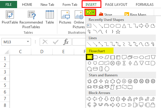
• In the "Illustrations" section, we must first select the "Shapes" drop-down under the "Insert" tab. The drop-down gives the options of all the shapes available, then choose the shape we need for the Excel flow chart and insert the shape on the worksheet.

To start with, let us insert the oval shape. Then, select the shape, keep the cursor, and drag it using the mouse to the size we want to see.

The above figure shows that the shape's size is adjusted and set within the gridlines as we have enabled the "Snap to Grid'' option. It will get changed while we start drawing the shape. When the shape is expanded or contracted, it will adjust to the nearest gridline.

• To add text to the shape, we must right-click and select the "Edit Text" option in the list.

• Insert the text in shape. We can align the text by using the text "Alignment" options.

We need to insert the next shape to proceed with the next step. Insert the next shape right below the "START." We can use the rectangle shape to show the stage where there is only one option to proceed further, and the diamond shape can be used when we have two or more options to proceed further.

The next step is to connect the shapes. Select the connector lines from the "Shapes" option and draw between the shapes to connect the shapes.

Once the connector is selected, keep the cursor on the shape, and we can see the connecting dots in shape.

Now, we must start drawing the line by dragging the mouse from any of the connecting dots and joining it with the connecting dot of the other shape. The connecting dots of the next shape can be seen while drawing the line close to the shape.

Keep adding the shapes one after the other as per the steps involved in the process.

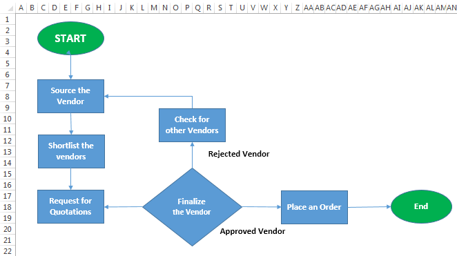
As we mentioned earlier, the diamond shape will be used where multiple options are involved. For example, in the above image, we can see the flow of the chart showing the different options associated with the diamond-shaped icon.

Each diagram shows only the step to be followed to complete the process. But for a clear understanding of the process, we can add additional information using the text box.

To add a text box,

• Go to the Insert Ribbon tab in excel and click the "Text box" from the “Text” Section.

• Now, we must insert the text box by keeping the cursor in place and dragging it using the mouse. Then finally, click inside the box to enter the text.

• Remove the outline by selecting the "Format Shape" (Do right click on the box for the option) and select "No Fill" from the "Format Properties."

Again, we can use an oval shape to show the end of the process.

• Remove gridlines by unchecking the "Gridlines" box in the "View" tab to make the chart look better.

Like this, the flow chart looks after completing all the steps.

We can format the shape of each step:

• Select the shape we like to format, go to the "Format" tab in the ribbon, click on the drop-down option in the "Shape Styles" section, and select the format.

Example #1 - Create Flow Chart Using Shapes (Step-By-Step)

Firstly let us build a flowchart of one popular flow chart, i.e., the organizational hierarchy chart. Below is the flow of communication in the organization.

President > Departmental Heads > Senior Manager > Manager > Team Leaders > Team Members.

It is the typical organization flow chart we usually get to see. In this article, we will learn to create a flow chart in Excel using shapes.

1. We must first remove gridlines from the worksheet.

    

2. Then, go to the Insert tab - Shapes - Flowchart - Rectangular shape.

   
   

3. Let us draw this first.

   
   
   
   Note: To fit column and row end, we must hold the "ALT" key and adjust.

4. After that, we must right-click and select "Edit Text."

   
   

5. Then, type the word "President."

   
   

6. This shape is not looking great. Therefore, under the "Format" option, we can change the format of the shape, as shown in the below image.

   
   

7. Now, the first position in the organization is over. Under "President," four departmental heads will come. For this, we must draw a straight line arrow.

   
   

8. We need to draw one horizontal line for all the departmental heads.

   
   

9. Now, we need to insert four more arrow lines.

   
   

10. Insert four more rectangular boxes under each arrow.

    
    
    
    Note: We have added four departments. We can alter it as per the requirement.

11. .Once the department heads' boxes are drawn, draw four more arrows and four more rectangular boxes for "Senior Manager."

    
    

12. . Under "Senior Manager," "Team Leader" will appear. Then, draw four more arrows and four more rectangular boxes for "Team Leader."

    
    

13. .Under each "Team Leader," four executives will come. But, first, we must draw one straight vertical line under each "Team Leader," as shown in the below image.

    
    

14. .We must draw four horizontal arrows for each vertical straight line. Therefore, we must draw 16 horizontal arrows.

    
    

15. . We must insert 16 text boxes in front of newly drawn horizontal arrows. For example, for the first box, type "Executive 1." For the second box, type "Executive 2." For the third box, type "Executive 3." And for the fourth box, type "Executive 4."

    
    

16. . So, now our flow chart for an organization is done. The flow of communication is clear in this chart. Each position in the organization is aware of whom they should contact to communicate their messages.

    
    

Example #2 - Create Business Flow Chart Using Smart Arts (Step-By-Step)

We have seen the steps for creating a typical Excel flow chart using shapes. Using SmartArt can make the flow chart look beautiful. The SmartArt flow chart is already predefined. If we need anything extra, we need to make arrangements.

In this example, we will explain establishing a new company.

• Step 1: We must first go to Insert - SmartArt.

• Step 2: Under the SmartArt, select "Process." Scroll down and select the "Repeating Bending Process."

• Step 3: Now, we have a default flow chart.

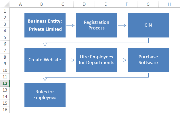
• Step 4: The advantage here is we have pre-drawn shapes. We must type "Business Entity Type: Private Limited" for the first box.

• Step 5: The next step is the "Registration Process."

• Step 6: Then, obtain the "Company Identification Number (CIN)."

• Step 7: The fourth step is to create a website for the company.

• Step 8: After that, we must hire employees from different departments.

• Step 9: We have two more steps to enter, but we do not have any shapes. So, we must select any one shape and paste it.

• Step 10: Now, we have inserted two more boxes. Type "Purchase Software" and "Rules for Employees" in the new boxes.

Example #3 - Design Flow Chart Using Excel SmartArts (Step-By-Step)

Now, we have all the processes in a flow chart. So let's design the SmartArt now.

• Step 1: First, we must select the "FlowChart Smart Art."
• Step 2: Two more tabs will appear in the ribbon as soon as we choose them. Select "Design."

• Step 3: Choose " Change Colors " under the "Design” tab, and choose "Change Colors."

• Step 4: Change the color of the SmartArt as per wish.

• Step 5: Change the flow chart style under the "Design" tab.

Example #4 - Using SmartArt Graphic

The flow chart can be created using Excel's readily available "SmartArt Graphic."

• We must first select the "SmartArt Graphic" in the "Illustrations" section under the "Insert" tab.

• Now, select the diagram as per the requirement and click "OK."

• After selecting the diagram, we must enter the text in the "Text Box."

The flow chart looks like as given below:

We can add the shape to the existing diagram. We can move up/down the shape in the "Design" tab by selecting the diagram.

Also, we can add shapes to the existing ones.

• We must use different shapes to create a flow chart in Excel to give visual effects.
• We must provide different colors to each tab while creating an Excel flow chart to make it more attractive.
• We must use the SmartArt graphics for an easy drawing of shapes.
• In the case of more complex flow charts, we must use shapes. Do not use SmartArt graphics.