Table Of Contents
What Is FIXED Excel Function?
The FIXED Excel inbuilt Text function helps round the given number to the cited number of decimals. The result is a number in the text format, with a period and commas.
Users can use the FIXED Excel Text function to make financial data in business reports and presentations more presentable. Also, the function helps round off currency values to the nearest denominations.
For example, the following dataset shows a number.
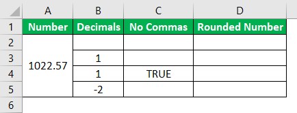
The requirement is to round the given number based on the decimal values and comma inclusion status specified in the dataset. Assume the target cells are in column D.
Then, we can use the FIXED Excel function in each target cell to achieve the required output.

In the above FIXED Excel function example, we supply the number, decimals and no comma requirement-based logical value, if cited, as the inputs to the FIXED Excel Text function.
Thus, the FIXED() returns the rounded number based on the input values.
For example, the FIXED Excel Text function in cell D4 accepts 1022.574, 1, and TRUE as the first, second, and third arguments. So, the function rounds off the given number to one decimal place and does not include a comma to mark thousands to return the text value 1022.6 as the output.
Table of contents
- The FIXED Excel Text function enables one to round off the given number to the specified decimals, with or without commas, and return the output as a text value.
- Users can use the FIXED function to make financial and statistical data appear more professional. Also, the function is useful for rounding currency values to the required denominations.
- The FIXED function accepts one mandatory argument, number, and two optional arguments, decimals and no_commas, as inputs.
- While we can use the FIXED function as a standalone function, using it with other inbuilt functions, such as CONCAT and IF, and operators, such as the ‘&’, yields fruitful results.
Syntax
The FIXED Excel formula syntax is as follows:

Where,
- number: The value we aim to round off and obtain in the text format.
- decimals: The count of digits we want after the decimal point.
- no_commas: It can be the logical value, TRUE or FALSE. We can supply it as TRUE if we do not want commas to appear in the FIXED Excel formula output text value.
While the first argument in the FIXED Excel Text function is mandatory, the remaining two are optional. Also, each argument can be a value, a FIXED Excel cell reference or a formula.
Furthermore, here are the rules to follow while supplying the FIXED Excel Text function to avoid errors:
- The significant digits in the number argument value cannot exceed 15, but the decimals argument value can be up to 127.
- The three arguments can take positive, zero, and negative values. If the decimals argument value is negative, the FIXED() rounds the given number before the decimal point. On the other hand, if the no_commas argument value is 0, the function considers the value as FALSE. However, the function considers the argument value as TRUE if the value is a non-zero number.
- If we do not supply the decimals and no_commas argument values to the FIXED(), they take the default values of 2 and FALSE. So, the function returns a text value with the number rounded to two decimals after the decimal point and with commas.
How To Use FIXED Excel?
We can use the FIXED Excel Text function in 2 ways:
- Access from the Excel ribbon.
- Enter in the worksheet manually.
Method #1 – Access From The Excel Ribbon
Select a target cell for output - The Formulas tab - The Text function group drop-down - The FIXED Excel Text function.
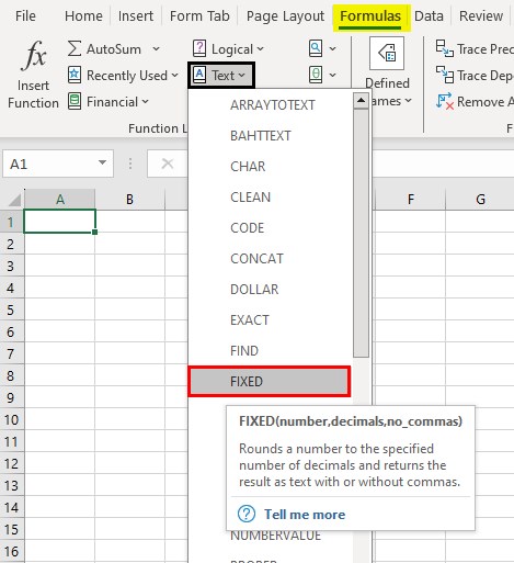
The Function Arguments window opens. Enter the arguments in the Number, Decimals, and No_commas fields - click OK, as depicted below.

Method #2 – Enter In The Worksheet Manually
- Choose a target cell for the output.
- Type =FIXED( in the cell.
- Enter each argument as a value, FIXED Excel cell reference, or a formula separated by commas and close the brackets.
- Press Enter to execute the FIXED Excel Text function and obtain the required rounded number as a text value.
Examples
Check out the following FIXED Excel Text function examples to use the function more effectively.
Example #1 - When ‘’ Argument Is Positive Or Negative
The following dataset contains numbers in column A.
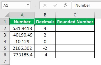
The requirement is to round off the given numbers to the decimals cited in the corresponding rows in column B and display the output in column C.
Then, here is how to use the FIXED Excel Text function in the target cells to achieve the required output.
Step 1: Choose cell C2 and enter the FIXED Excel Text function.
=FIXED(A2,B2)
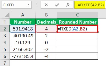
Step 2: Press Enter to implement the function in the target cell.
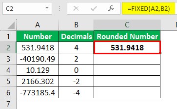
Step 3: Using the Excel fill handle, update the formula in the remaining target cells.
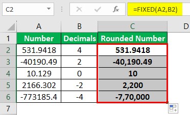
We shall check the FIXED Excel row 6 function in cell C6 to understand the logic.
The FIXED() accepts the references to the cells A6:B6 as the number and decimals argument values. Next, the second argument, decimals, is negative. So, the function rounds off the given number before the decimal point. Also, as we did not mention the no_commas argument value, the function takes its default value of FALSE.
Thus, the function rounds off the value -773185.37 before the decimal point by 4 decimals and returns the text value of -770,000 as the output.
Example #2 - If The ‘’ Argument Is TRUE Or FALSE
The following dataset shows the total annual sales at three branch offices of a firm.

The task is to round off the total annual sales figures to the default two decimals, and the resulting text values must include commas based on column C data in each row. Assume the target cells are in column D.
Step 1: Choose cell D2, enter the FIXED Excel Text function, and press Enter.
=FIXED(B2,,C2)
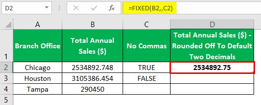
Next, using the fill handle, update the formula in cell D3.
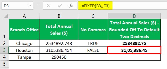
Step 2: Choose cell D4, enter the FIXED Excel Text function, and press Enter.
=FIXED(B4)
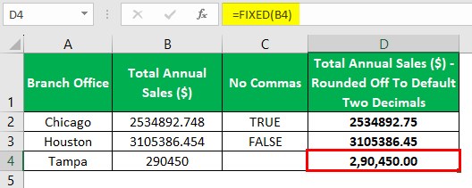
The FIXED() in the first two target cells accepts the cell reference to the total annual sales figures of the corresponding branch offices as the first argument value. Next, since the second argument must take its default value, we shall leave it blank. Finally, we supply the cell reference to the logical value in the corresponding row in column C as the third argument value.
Thus, the FIXED() in the two target cells returns the total annual sales figures as text values, rounded to two decimals. But since the third argument value in the first target cell’s FIXED() is TRUE, the first text value contains no commas. On the other hand, the third argument value in the second target cell’s FIXED() is FALSE. So, the second text value contains commas.
Furthermore, the FIXED() in the third target cell accepts only one input, the cell reference to the total annual sales figure of the corresponding branch office as the first argument value. The second and third arguments take their default values of 2 and FALSE.
Thus, the FIXED() returns a text value, with the total annual sales figures rounded to two decimals and including commas.
Example #3
The following dataset lists constants commonly used in Physics.

The task is to display the values rounded to three decimals, with commas included, and as texts, including the comments and units, if mentioned in column C rows.
Then, we can use the ‘&’ symbol with the FIXED Excel function in the target cells to achieve the required output.
Step 1: Choose cell D2, enter the following formula, and press Enter.
=A2&FIXED(B2,3,FALSE)&" "&C2

Step 2: Using the fill handle, update the formula in the remaining target cells.

Let us check the cell D5 formula to understand the logic.
First, the FIXED() accepts three arguments as input. While the first argument value is the reference to cell B5, containing the constant 0.0529, the second is 3, indicating the decimals to which we aim to round off the cited value. Finally, the third argument value is FALSE, indicating the resulting text value includes commas.
So, the FIXED() output will be 0.053.
Next, the formula concatenates the comment in cell A5, the FIXED() output, a space character, and the unit in cell C5 to return a text as the output, highlighted in cell D5.
Important Things To Note
- Ensure the first two arguments in the FIXED Excel Text function are numbers, and the third is the logical value, TRUE or FALSE. Alternatively, we can supply the third argument as 0 for FALSE and any non-zero number for TRUE. Otherwise, the FIXED() will return the #VALUE! error.
- If the number argument value exceeds 15 digits, Excel will replace the digit after the 15th digit with 0. On the other hand, the decimals argument value can be a maximum of 127 and a value beyond 127 will result in the FIXED() returning the #VALUE! error.
Frequently Asked Questions (FAQs)
We can use VBA FIXED in Excel using the following method:
Application.WorksheetFunction.Fixed(Arg1,Arg2,Arg3)
Arg1, Arg2 and Arg3 are the arguments number, decimals, and no_commas explained in the above article.
Let us see how to use the method with an example.
The following dataset contains numbers, and we must round them based on the specified decimals and commas requirements and display the output in column D.
Then, here is how to use the FIXED function in Excel VBA to achieve the required outcome.
Step 1: Open the sheet containing the above-shown dataset and press Alt + F11 to access the VBA Editor.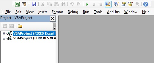
Step 2: Select the applicable VBAProject and choose Module under the Insert tab.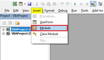
A new module window will appear.
Step 3: Enter the VBA code in the module window to apply the FIXED() in the target cells.
Sub FIXED_Fn()
Dim ws As Worksheet
Set ws = Worksheets("FIXED_FAQ")
ws.Range("D2") = Application.WorksheetFunction.Fixed(ws.Range("A2"), ws.Range("B2"), ws.Range("C2"))
ws.Range("D3") = Application.WorksheetFunction.Fixed(ws.Range("A3"), ws.Range("B3"), ws.Range("C3"))
ws.Range("D4") = Application.WorksheetFunction.Fixed(ws.Range("A4"), ws.Range("B4"), ws.Range("C4"))
End Sub
Step 4: Press the play icon in the top menu to execute the VBA code.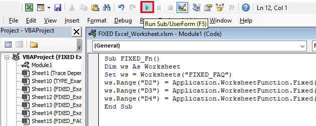
Finally, open the active worksheet to view the output in the target cells.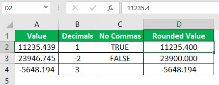
The FIXED() in each Column D target cell accepts the columns A:C cells in the corresponding rows as inputs to return the required rounded values as text values.
The difference between formatting a cell containing a number by using a command and formatting a number directly with the FIXED function is that the FIXED() converts the output to text.
The difference between rounding functions and the FIXED formula in Excel is that the rounding functions’ output is a number, which we can use in mathematical evaluations.
On the other hand, the FIXED() output is a text value, which we cannot use in mathematical calculations.
Download Template
This article must be helpful to understand the FIXED Excel, with its formula and examples. You can download the template here to use it instantly.
Recommended Articles
This has been a guide What Is FIXED Excel. We learn the FIXED Excel function syntax and how to use it with examples and points to remember. You can learn more from the following articles –
