Filter Shortcut in Excel

Excel Filter Keyboard Shortcut

In Excel, sorting and filtering data is a very important and common task. With the use of this, we can see the data category wise. For example, if you want to see the data/record of a class subject wise or sales data from the dozen of stores that you need to keep track of, you will be able to find the data quickly that you need.

With filtering data quickly, you can easily navigate through menus or clicking through a mouse in less time. In this article, we discuss keyboard excel shortcuts used for the filter.

How to Use Keyboard Shortcut For Filter in Excel?

Let us understand Filter Shortcut in Excel with the below examples.

Example #1 – Turn Filters ON or OFF in Excel

We have given below sales data region wise.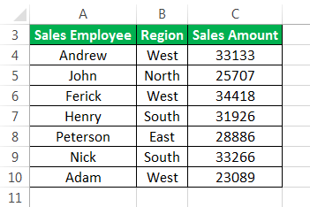

For this, follow the below steps:

• First, select a cell in your data range if the data range contains any blank columns or rows, then better to select the entire range of cells.

• Go to the DATA tab; then, click on the Filter option under the Sort & Filter section. Refer to the below screenshot.

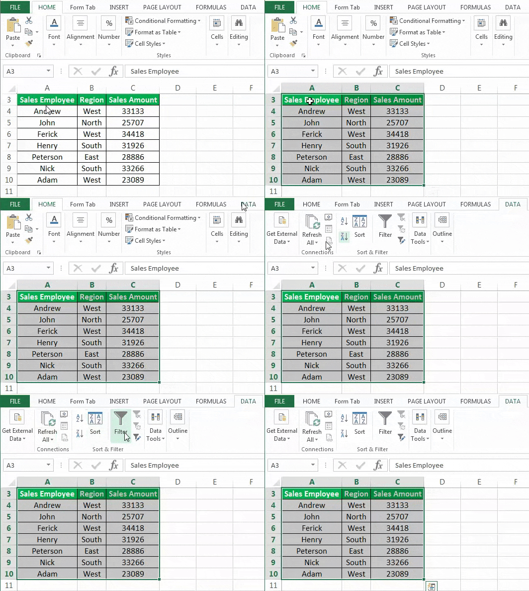
• We also can use the Keyboard Shortcut CTRL+SHIFT+L for turning On/Off the filters.

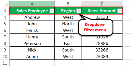
• Once applying the filter, the drop-down filter menus will appear in the header row of your data. Refer to the below screenshot.

Example #2 – Opening the Drop-down Filter Menu in Excel

Once the filter has enabled on your data, you can use the drop-down menus on each of the column headers. Follow the below steps for doing this:

• Select a cell in the header row. As we can see that every cell contains drop down an icon like the image then, Press the ALT + down arrow key on the keyboard to open the filter menu like the below screenshot.

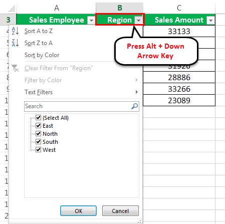
• As we can see in the above image, there are a lot of keyboard shortcuts available in the filter menu.

Example #3 – Select Menu Items Using Arrow keys

Once the excel filter is enabled, we can use arrow keys to navigate the filter menu. Use Enter and Spacebar key to select and apply to filter. Remember the below points:

• Press the Up and Down arrow keys to select a command.
• Press Enter Key to apply the command.
• Press the Spacebar Key to check and uncheck the checkbox.

Example #4 – Drop Down Menu Keyboard Shortcut for Filter in Excel

You must first press the ALT+ Down Arrow key to display the drop-down menu. With this, you can one of the following:

• S – Sort A to Z
• O – Sort Z to A
• T – Sort by Color submenu
• C – Clear filter
• I – Filter by Color submenu
• F – Text Filters
• E-Text Box

Example #5 – Clear All Filters in the Current Filtered Range in Excel

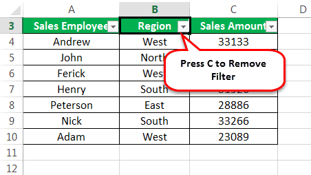
Press shortcut key ALT+Down Arrow+C to clear all the filters in the current filtered range. It will clear all the filters in all the columns. After that, all rows of your data will be displayed.

For this, you also can use the Excel ribbon option.

Example #6 – Clear Filter in a Column

To clear filter in a column, follow below steps:

• Select a cell in the header row and press Alt+Down Arrow to display the filter menu for the column.

• Press the letter “C” to clear the filter.

Example #7 – Display the Custom Filter Dialog Box

When you want to filter the data by using custom criteria, you can use a custom filter box. For this, follow the below steps:

• Select a cell in the header row.
• Press the ALT+Down Arrow key to display the filter menu for the column.
• Type the letter “F.”
• Type the letter ”E.”
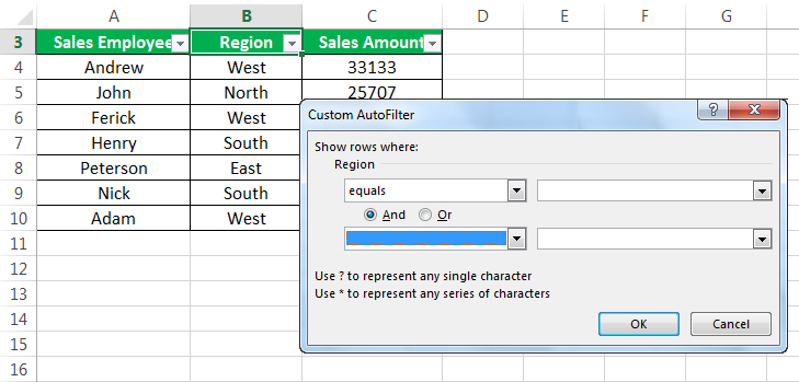
• Then a custom dialog box will appear, which sets the comparison operator to equal. See the below screenshot.

• Select the option from the list (such as not equal, etc.) and enter the criteria.

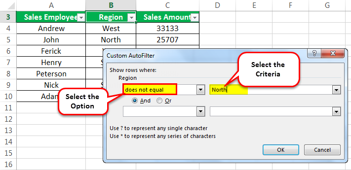
• Select And or Or then Press OK to apply the filter.

It Displays Filtered Data.

Things to Remember About Filter Shortcut in Excel

• If you are using the Excel tables feature, then you can apply the filters on more than one table range at a time in the same worksheet.
• Using filters keyboard shortcut in excel, you can save a lot of time.
• Use the keyboard shortcuts, as explained in this article, are the fastest way to work with the filter menus.

Recommended Articles

This has been a guide to Filter Shortcut in Excel. Here we discuss how to use keyboard shortcuts for a filter in excel in different ways along with practical examples and downloadable excel templates. You may learn more about excel from the following articles –

• How to Add and Use Filter in Excel?
• Advanced Filter in Excel
• Auto Filter In Excel
• AutoFill in Excel