False In Excel

The FALSE function in Excel is a logical function that returns "FALSE" as an output when used in a blank cell. This function also does not take any arguments similar to the TRUE function in Excel. Instead, it is used with the other conditional functions, such as the IF function, to return a "FALSE" as a value if the condition is met or not.

For example, consider the below example showing a value in cell B1.

Now, let us find whether the value is more than 1000 or not using FALSE function in Excel.

The steps are:

Step 1: First, enter the function, =B1>1000

Step 2: Next, press Enter.

We can see the result as shown in the below image.

Likewise, we can use FALSE function in Excel.

• FALSE function in Excel provides a "FALSE" result when it is utilized in an empty cell. It is usually utilized with other conditional functions, such as IF, to return a "FALSE" value based on a condition.
• This function in Excel is equivalent to 0 and allows for mathematical operations. If any number is multiplied by this function, it will result in zero.
• The FALSE function returns "FALSE". FALSE and FALSE() are the same, with a 0 value. No arguments are needed for the function.

Below is the FALSE formula in Excel.

The FALSE formula in Excel requires no arguments.

One may also enter the word "FALSE" directly into any cell or formula, and Excel will interpret this as the logical value "FALSE."

It is mostly used in conjugation with other functions, such as conditional functions, which do different things depending on whether a certain criterion is met. For example:

1. An employer will increase your monthly payment if you have reached a particular target.
2. You will get a discount coupon only when you have done shopping for more than $5,000.

The FALSE function in Excel is equivalent to the number 0. We can perform all the mathematical operations with this function. If we multiply any number with this function, it will return zero.

Example #1

To obtain a FALSE in a cell, we must enter the FALSE function :

=FALSE()

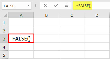
Press the "Enter" key.

The function will return "FALSE."

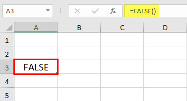
We can use the function along with mathematical operations, in which the function takes the value 0. Let us see an example.

Example #2

Suppose we multiply a number, e.g., 10, with the function. The syntax will be:

=FALSE * 10 or FALSE() * 10

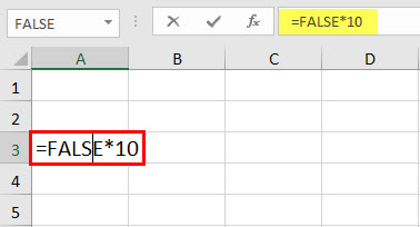
Press the "Enter" key.

The function will return 0.

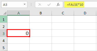
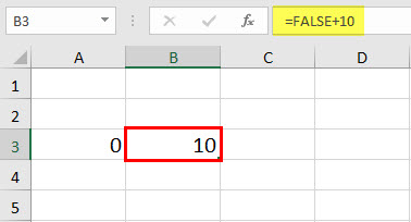
Similarly, if we add the number with the function,

Syntax: =FALSE + 10 or FALSE() + 10

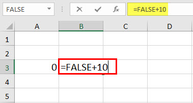
Consequently, it will return 10 (as 0+10=10).

Example #3

Suppose we have a number in cell C3, and we want to check whether the number is greater than 50.

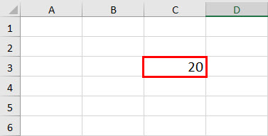
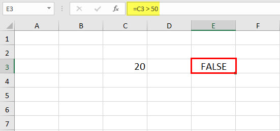
We can use the following syntax to check the condition.

=C3 > 50

The syntax will return "FALSE".

Similarly, we can check if the number in C3 is less than 10 using the syntax below.

=C3 < 10

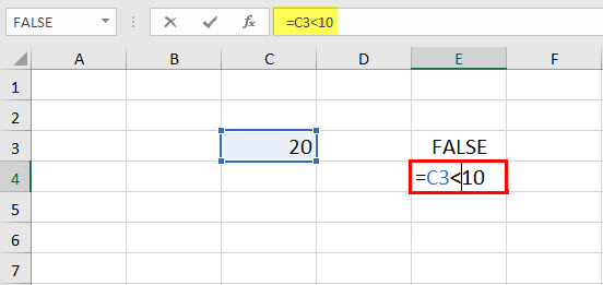
Again, this returns "FALSE."

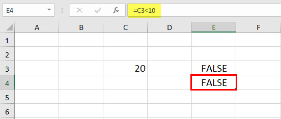
The FALSE function is most widely used with conditional functions. Let us see an example of using a FALSE function with an IF condition.

Example #4

Suppose different employees in your company sell the same item. Then, depending on the number of items an employee sells in a month, we will decide whether to give the employee a bonus or not. For example, five employees' number of items sold (A4: A8) is shown in B4: B8.

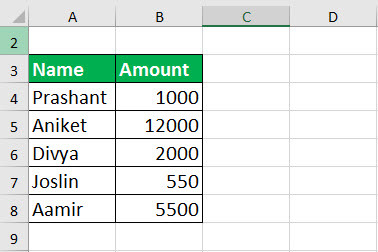
If an employee sells equal to or more than 1,000 goods, he will get a bonus. So, the syntax for the first employee would be:

=IF(B4>=1000, TRUE, FALSE)

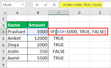
It returns "TRUE" when the employee has reached the target and "FALSE" when they have not.

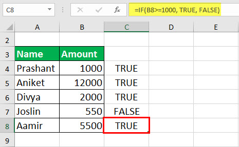
The IF function works on the logical values "TRUE" and "FALSE." We may note here that if we do not provide the value_if_false in the IF function, it will automatically return "FALSE," as shown below.

Example #5

Suppose you run a delivery outlet. In this, you maintain a sheet of order numbers and their delivery status, as shown below.

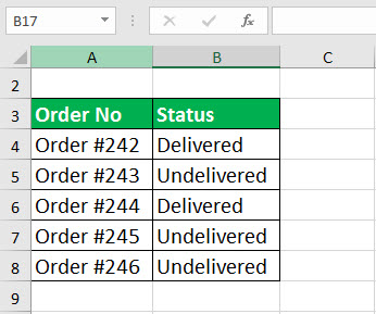
So, if the status is "Delivered," the order is complete. We can check whether an order is complete or not using the FALSE statement. For example, for the first order (given in A4:B4), we can use the syntax:

=IF(B4=” Delivered”, TRUE, FALSE)

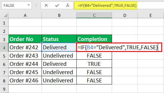
Expanding the function to the rest of the cells will return the completion status in "TRUE" or "FALSE."

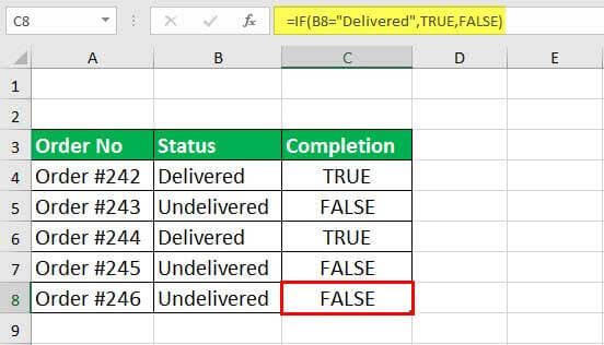
We may also calculate the number of pending orders using the function COUNTIF as:

COUNTIF(C:C,FALSE)

The function will count the number of times the value "FALSE" occurs in column C.

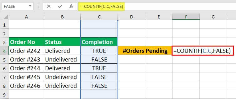
Since the number of "FALSE" in this example is 3, it will return 3.

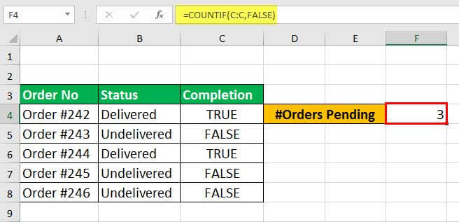
Instead of C:C, we may also use C4:C8 since the values are in these cells only. However, the entries may keep increasing with time. Therefore, it will not be required to change every time an entry is added for C: C.

Example #6

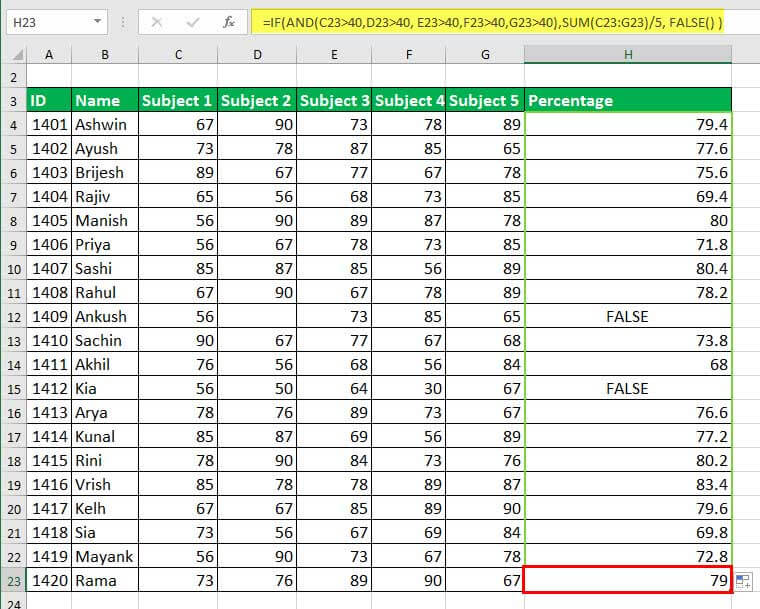
Suppose we have a list of students and their marks in 5 different subjects.

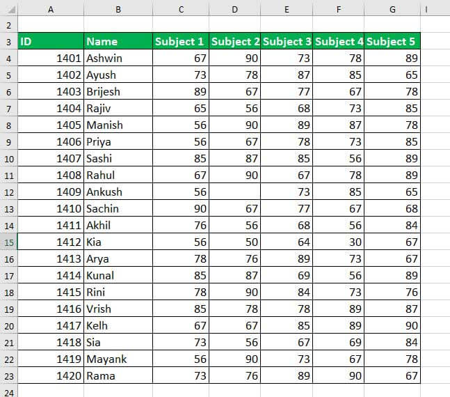
If any cell for marks (C4: G23) is left blank, it specifies that the student has not given the exam. If the marks are less than 40, the student is considered to fail. In both cases, the student's final result is not declared. So now, we can calculate the percentage of the students who have successfully passed all the subjects but not those who could not.

We may use the following syntax:

=IF(AND(C4>40, D4>40, E4>40, F4>40, G4>40), SUM(C4:G4)/5, FALSE )

In this syntax,

1. AND(C4>40, D4>40, E4>40, F4>40, G4>40)

It will return "TRUE" if the student has scored marks greater than 40 in all the five subjects. Else, "FALSE."

2. IF(AND(…), SUM(C4:G4)/5, FALSE )

which implies

=IF(TRUE,SUM(C4:G4)/5, FALSE )   or  =IF(FALSE,SUM(C4:G4)/5, FALSE )

If AND(…) returns "TRUE," the IF function will return the percentage of marks the student has secured, SUM(C4: G4)/5.

If AND(…) returns "FALSE," the IF function will also return "FALSE."

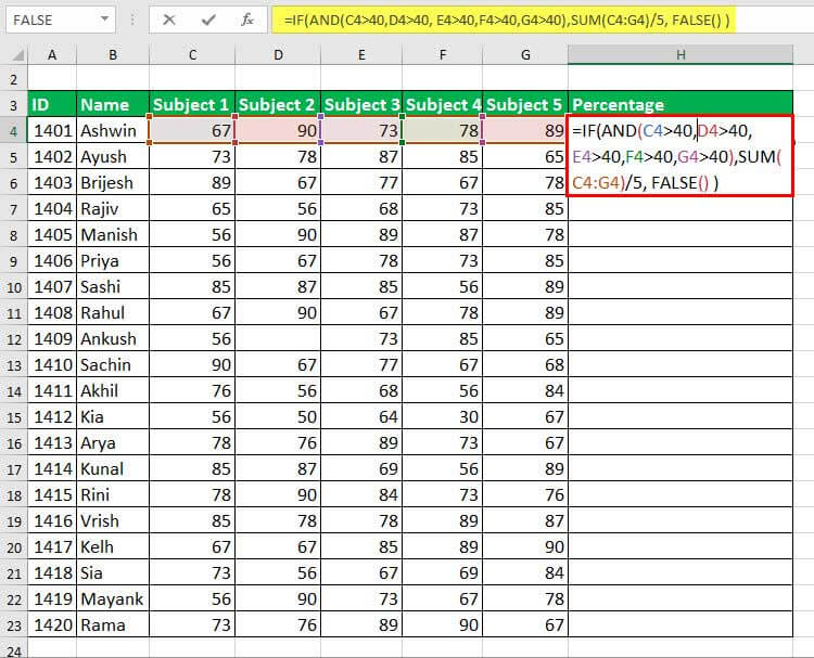
We can drag it to the rest of the cells and will get the final output as:

Since it is a logical value, "TRUE" is the opposite of "FALSE." Therefore, if we type NOT(FALSE), it will return "TRUE." See the example below.

Example #7

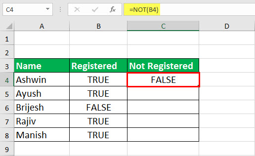
Suppose we have a list of interested participants for the campaign and the information on whether they have registered or not, as shown below.

If it says, "Ashwin has registered," we will say "TRUE." However, if it says, "Ashwin has not registered," we will say "FALSE." We may change "TRUE" to "FALSE" by using the NOT function in excel.

For the first name in the list, the syntax will be:

=NOT(B4)

It will return "FALSE".

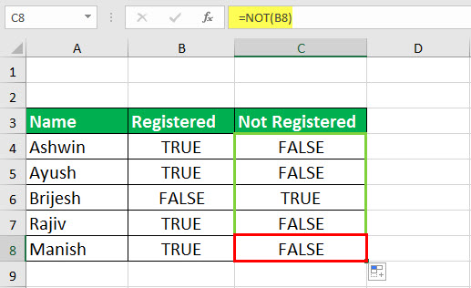
As shown below, we can drag it to the rest of the cells. We may get the final output for the complete list.

• The function returns the logical value "FALSE."
• The FALSE and FALSE () both are identical.
• The FALSE function has a value of 0.
• There are only two logical values: TRUE and FALSE. TRUE is the opposite of FALSE.
• The function does not require any argument.

This article has been a guide to the FALSE Function in Excel. We discussed the FALSE formula in Excel, using the FALSE function and Excel examples, and downloadable Excel templates. You may also look at these useful functions in Excel: -

• Top Shortcuts for SUM in Excel
• VBA DIR Function
• ISBLANK() Function in Excel
• RANKX Function in Power BI