Exponential Distribution

The exponential distribution is a continuous probability distribution that times the occurrence of events. These events are independent and occur at a steady average rate. In other words, it is used to model the time a person needs to wait before the given event happens.

It is a continuous counterpart of a geometric distribution. It is a memoryless random distribution comprising many small values and less large values. It is different from the Poisson distribution — Poisson predicts the number of times an event transpires in a given period and not the time gap.

• The exponential distribution is a probability distribution that anticipates the time interval between successive events. The events should occur continuously and should be independent of each other.
• This memoryless random distribution facilitates the estimation of an event's occurrence, success, or failure.
• It is calculated as:

• Here x denotes the random variable, and λ is the scale parameter—the reciprocal value of the mean.

In statistics, the exponential distribution function determines the constant rate of time-lapse between the occurrence of two independent and continuous events.

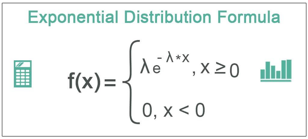
Let us assume, x is a continuous random variable (scale parameter λ > 0). The variable x can have an exponential distribution if it meets the following requirement:

A researcher should be able to express the probability density function of x by multiplying the scale parameter by the exponential function of the minus scale parameter and x (for all x greater than or equal to zero).

If x does not meet the conditions, the probability density function is equal to zero.

In statistics, this concept is used for predicting events' success, failure, or occurrence. For example, the concept can anticipate the time a potential customer will take to buy a product or service. Similarly, it can determine the frequency of buses at a particular stop or the frequency of earthquakes per year.

Mathematically, the probability density function is represented as:

Here, f (x; λ) is the probability density function,

λ is the scale parameter which is the reciprocal of the mean value,

x is the random variable.

Follow the below steps to determine the exponential distribution for a given set of data:

1. First, decide whether the event under consideration is continuous and independent. Ascertain if it occurs at a roughly constant rate. For all practical events, the variable should be greater than or equal to zero.
2. Next, determine the value of the scale parameter. It is invariably the reciprocal of the mean; λ = 1 / mean.
3. Next, multiply the scale parameter λ and the variable x.
4. Now, calculate the exponential function of the product multiplied by minus one, i.e., e^-λx.
5. Finally, calculate the probability density function by multiplying the exponential function and the scale parameter.
6. If the above formula holds true for all x greater than or equal to zero, then x is an exponential distribution.

Similarly, we can compute the following:

• Mean of Exponential Distribution: The value of lambda is reciprocal of the mean, similarly, the mean is the reciprocal of the lambda, written as μ = 1 / λ.
• Median of Exponential Distribution: Median can be determined as the fraction of the natural value of log (2) by lambda, written as M = log (2) / λ.
• Variance of Exponential Distribution: The variance is determined with the help of the exponential distribution's second moment and is denoted as follows:
  Var (x) = 1 / λ ²

Let us determine the amount of time taken (in minutes) by office personnel to deliver a file from the manager's desk to the clerk's desk. The function of time taken is assumed to have an exponential distribution with the average amount of time equal to 5 minutes. Also, x is a continuous random variable. Based on the given data, determine the exponential distribution.

Given:

x = time taken to deliver a file in minutes

μ = 5 minutes

Therefore, scale parameter is:

λ = 1 / μ

λ = 1 / 5 = 0.20

Hence, the exponential distribution probability function can be derived as,

f (x; λ) = 0.20 e ^{– 0.20*x}

Now, calculate the probability function at different values of x to derive the distribution curve.

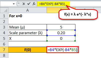
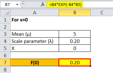
For x = 0

Exponential distribution probability function For x=0 will be,

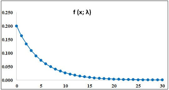
Similarly, calculate exponential distribution probability function for x=1 to x=30

• For x = 0, f(0) = 0.20 e ^-0.20*0 = 0.200
• For x = 1, f(1) = 0.20 e ^-0.20*1 = 0.164
• For x = 2, f(2) = 0.20 e ^-0.20*2 = 0.134
• For x = 3, f(3) = 0.20 e ^-0.20*3 = 0.110
• For x = 4, f(4) = 0.20 e ^-0.20*4 = 0.090
• For x = 5, f(5) = 0.20 e ^-0.20*5 = 0.074
• For x = 6, f(6) = 0.20 e ^-0.20*6 = 0.060
• For x = 7, f(7) = 0.20 e ^-0.20*7 = 0.049
• For x = 8, f(8) = 0.20 e ^-0.20*8 = 0.040
• For x = 9, f(9) = 0.20 e ^-0.20*9 = 0.033
• For x = 10, f(10) = 0.20 e ^-0.20*10 = 0.027
• For x = 11, f(11) = 0.20 e ^-0.20*11 = 0.022
• For x = 12, f(12) = 0.20 e ^-0.20*12 = 0.018
• For x = 13, f(13) = 0.20 e ^-0.20*13 = 0.015
• For x = 14, f(14) = 0.20 e ^-0.20*14 = 0.012
• For x = 15, f(15) = 0.20 e ^-0.20*15 = 0.010
• For x = 16, f(16) = 0.20 e ^-0.20*16 = 0.008
• For x = 17, f(17) = 0.20 e ^-0.20*17 = 0.007
• For x = 18, f(18) = 0.20 e ^-0.20*18 = 0.005
• For x = 19, f(19) = 0.20 e ^-0.20*19 = 0.004
• For x = 20, f(20) = 0.20 e ^-0.20*20 = 0.004
• For x = 21, f(21) = 0.20 e ^-0.20*21 = 0.003
• For x = 22, f(22) = 0.20 e ^-0.20*22 = 0.002
• For x = 23, f(23) = 0.20 e ^-0.20*23 = 0.002
• For x = 24, f(24) = 0.20 e ^-0.20*24 = 0.002
• For x = 25, f(25) = 0.20 e ^-0.20*25 = 0.001
• For x = 26, f(26) = 0.20 e ^-0.20*26 = 0.001
• For x = 27, f(27) = 0.20 e ^-0.20*27 = 0.001
• For x = 28, f(28) = 0.20 e ^-0.20*28 = 0.001
• For x = 29, f(29) = 0.20 e ^-0.20*29 = 0.001
• For x = 30, f(30) = 0.20 e ^-0.20*30 = 0.000

Based on data, the following distribution curve is derived:

In exponential distribution, the number of large values is much smaller than the small ones, which reflects a nearly constant time lapse between the events. The assumption of a regular rate is very rarely satisfied in real-world scenarios. But, if the selected time interval is roughly constant, then the exponential distribution can be used as a good approximate model.

It is one of the extensively used continuous distributions, and it is strictly related to the Poisson distribution in excel. The continuous probability distribution is used for time modeling, reliability modeling, and service time modeling. The concept has extensive application in statistics, physics, hydrology, disaster management, and business.

This article has been a guide to Exponential Distribution. We explain exponential distribution meaning, formula, calculation, probability, mean, variance & examples. You can learn more about statistical modeling from the articles below –

• Formula of T Distribution
• Binomial Distribution Formula
• Uniform Distribution
• Probability Distribution Examples
• Rule of 70