VLOOKUP With SUM

VLOOKUP, or Vertical Lookup, is a very versatile function that we can combine with other functions to get some desired result. VLOOKUP with SUM helps us calculate the sum of the numeric values based on the matching criterias or conditions.

To perform VLOOKUP with SUM, we combine two built-in Excel functions, i.e., SUM() and VLOOKUP(), to get the following syntax,

=SUM(VLOOKUP(lookup_value, table_array, col_index_num, ).

For example, we will find the February bonus for an employee from the employee bonus data table given below.

Enter the formula =SUM(VLOOKUP(F2,$A$2:$D$7,{3,4,5},0)), and press “Ctrl+Shift+Enter” to execute the formula as an array.

The total bonus earned by the employee “Sumit Bala” in 3 months is $10,870.

We need to understand the various terms associated with using VLOOKUP and SUM in Excel to find the total values that meet the criteria.

The formula should be entered as follows: SUM(VLOOKUP(lookup_value, table_array, col_index_num, and range_lookup))

The four elements to be considered are,

• lookup_value – It is the value we search for to determine the sum that matches exactly. It changes the lookup_value to determine the sum of different columns using different criteria.
• table_array – It is the range of cells helpful to search for data using the specified criteria. Generally, it will be a table of data generated from different sources.
• col_index_num – To find, we should enter the sum of the array of indexes. One can enter all or a few column indexes based on the requirement. These are helpful in the identification of the columns, including in sum.
• range_lookup – Appropriate logic value, either 0 and 1 or “True” or “False” to select the values that match or approximately.

Below are some examples of VLOOKUP with the SUM function.

Example #1

Use of simple SUM and the VLOOKUP function.

The sales of the laptop are determined using the SUM and VLOOKUP, which can also be done simply using the sum formula. The reason for using VLOOKUP with SUM is the feasibility of changing the lookup_value of cell G3 to determine sales of other items like “DVDs” and “Phones”. By changing the lookup_value to the phone, sales of the phone are generated, as shown below.

In the present scenario, the VLOOKUP function eliminated individual calculation of the sum of sales produced.

Example #2

Determining the sum of sales generated in two different worksheets using Excel VLOOKUP and SUM. Consider the following data to explain this example.

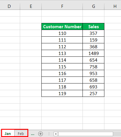
Three worksheets are created, including Jan, Feb, and summary, to determine the total sales generated by a customer. In this, two VLOOKUP functions are added for two worksheets, January and February, to determine the total sales as shown in the below-mentioned figure.

For determining the sales generated by other customers, the formula is dragged to other rows by adding absolute cell reference to the range of data. It will produce accurate results in the use of SUM and VLOOKUP.

Example #3

Summing of values presented in alternative columns

It is possible to sum the values shown in alternative and specified columns. The following table is considered to illustrate the present example.

Suppose we want to determine the sum of values in alternative columns, including January, March, May, July, September, and November. To do this, indexes of only these columns should be considered instead of all column indexes, as shown in the below screenshot.

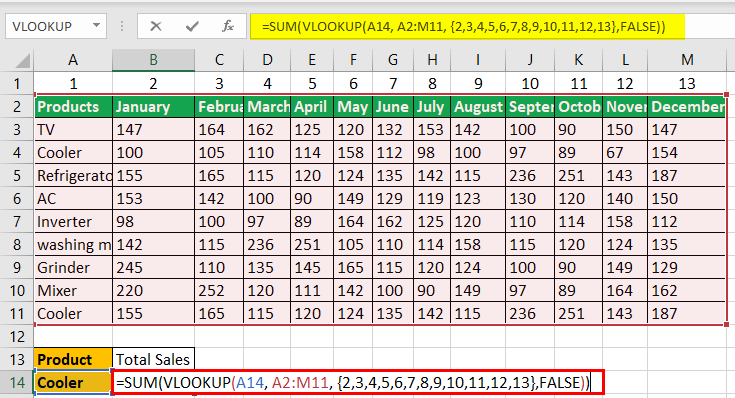
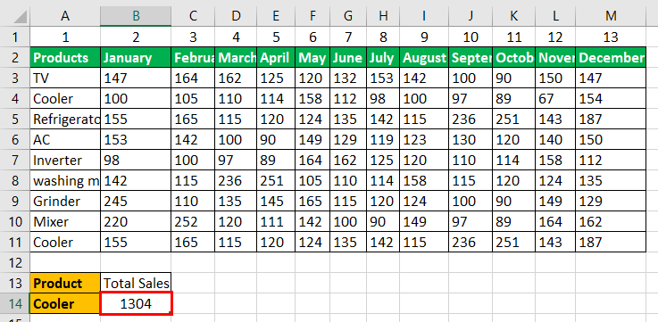
To get sales of other products, simply change the value in cell B14. It helps get the desired result. Therefore, it is the best feature provided by Excel VLOOKUP, as shown below.

We can use VLOOKUP With SUM function by,

1. Determining the sum of matching values in columns.
2. Determining the sum of matching values in rows.

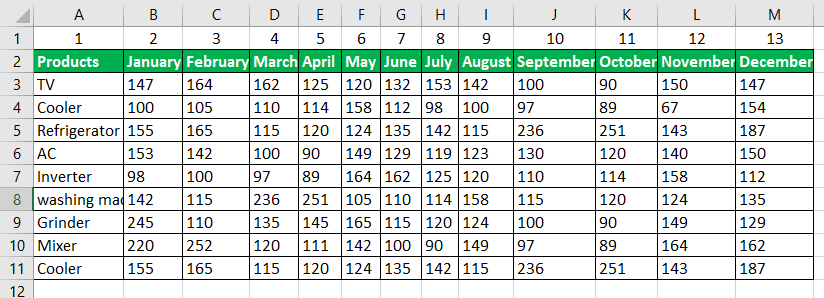
The table is created for understanding, as shown in the figure below.

#1 – Determining the sum of matching values in columns

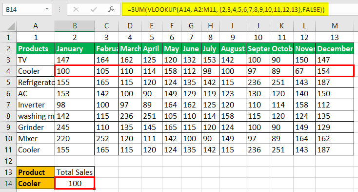
If we want to determine the total sales of the cooler from January to December, we should enter the specific criteria into the empty cell.

In this, the lookup_value is presented in the cell called A15, and A2:M11 is the range of data. The numbers 2 to 13 are the indexes for the columns. Applying these to the Excel VLOOKUP and SUM formula will obtain the sales cooler’s total value. After entering the formula, press the “CTRL+SHIFT+ENTER” keys at a time to yield the result. Otherwise, only the first cell’s value is displayed without all the values. This process applies to the remaining products to find the sum of values in different columns.

#2 – Determining the sum of matching values in rows

The below-mentioned sheet shows the sales of the cooler in the different rows. These are summed using the SUMPRODUCT function.

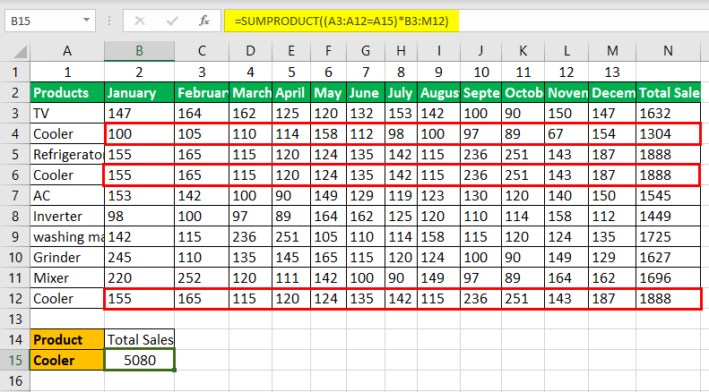
In this, the lookup_value is presented in cell A15, which is considered as a criteria to determine the sum of sales. We can change this value to other products to find out the sales. But, in this process, simply pressing or entering after writing the formula yields better results.

• We should create the name for a range of cells or arrays with VLOOKUP. It needs to ensure that the lookup value is placed in the first column for the proper working of VLOOKUP.  
• Ensure to give the right index numbers to the columns to be easily used. For example, the lookup_value column is indicated with 1, the next column with 2, and so on.
• We should enter the appropriate logical value, either “True” or “False,” to the approximate or exact match of a lookup_value, col_index_num, and range of cells to avoid errors.