Excel Paste Transpose

Last Updated :

Blog Author :

Edited by :

Reviewed by :

Table Of Contents

Paste Transpose in Excel

In Excel, there are instances that you would have never imagined before. But if you are good at advanced skills, you will find a way to sort it out. One such instance as a new user we face is “Transposing the data.” The word Transpose may be strange, but this will be the feature you may have to use more often than not to organize the data. So in this article, we will show you different ways of pasting and transposing the data in Excel.

Paste Transpose in Excel

What is Transpose in Excel?

In Excel, we store data in rows and columns. It depends on the user how they want to show the data. For example, some users may want to see more rows than columns, and others may wish to see more rows than rows. So in these cases, we can change the position of the rows into columns and columns into rows.

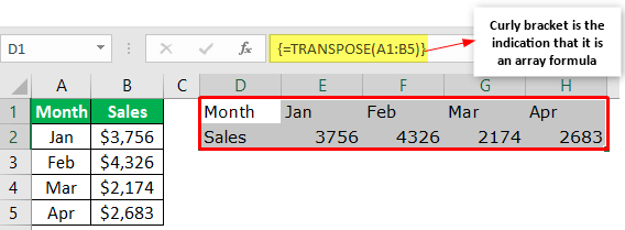
So the process of swapping columns with rows is called “Transpose in Excel.” Below is the image of the transposed data.

So, now we will see how we can transpose by using different methods.

Two Ways to Paste Transposing Data in Excel

There are mainly two ways to use Excel to swap rows and columns. Those two methods are below.

#1 - TRANSPOSE Function

Looking at the list of formulas in Excel, we have a function called “TRANSPOSE” under the “Lookup & Reference” category. It is an array formula, so using this function, we can interchange the position of rows and columns of data.

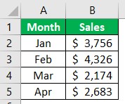
For example, look at the below data.

We need to transpose the above data. So to use the TRANSPOSE function, we need to do a little bit of work before, i.e., counting the number of rows and columns in the current table.

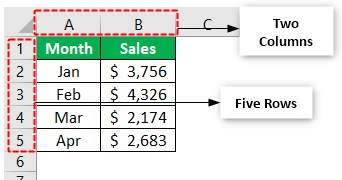
We have two columns and five rows of data in the current table.

Before we use the TRANSPOSE function, we need to select five columns and two rows. Yes, because we are transposing the data, we need to choose the opposite number of rows and columns in transpose.

Because of a current number of rows, data will come to a column, and current columns data will come to rows. So, in this case, we have five rows in the current table, so select five columns in the new table. We have two columns in the current table, so select two rows in the new table.

Look at the above picture; we have selected five columns and two rows (D1 to H2). Now, open the TRANSPOSE function in the D1 cell.

Choose the data range as the current table from A1 to B5.

TRANSPOSE is an array formula in excel, so we need to close the formula by holding “Ctrl + Shift + Enter” together.

Now, we have got the transpose of our data.

#2 - Paste Special Method

If you have used the paste special methods, you may know how good that tool is. We can transpose the data quickly and quicker than the TRANSPOSE method using the Paste Method.

Below given are the steps to transpose data using Paste Special Method.

First, we must copy the data range we need to transpose, so copy the table first.
Now select the cell where we must transpose the copied data to choose the D1 cell.
Now, right-click and hover on “Paste Special” to see paste special options.
From the above options, choose the method as “Transpose.”
Click on that, and it will transpose data.
The even quicker way is following the shortcut method. After copying the data, we must press the paste special shortcut key ALT + E + S to open the Paste Special method.
Choose “Transpose” as the “Operation” from the above window.
Click on "OK," and it will transpose data instantly.

To select the "Transpose" option in the "Paste Special" window, press "E" as the shortcut key. It will immediately choose the "Transpose" option.

Things to Remember

The TRANSPOSE function is directly linked to cells so that any changes will also reflect in transposed data.
The Paste Special method is not cell-linked. So we may not get any updated results in the transposed range.
With the Paste Special method, we may get exact formatting as in the main table, but we will not get any formatting with the TRANSPOSE formula.