Table Of Contents
Excel Group by Sum
While working with Excel, we get many new scenarios that have not been imagined. To Excel daily users, we should be able to encounter those scenarios. Of course, we cannot pinpoint any situation, but those unique situations will surely arise. One of the particular situations we have faced recently was getting the sum of multiple line items into one cell when we have all the line item values in one column. So in this article, we will show you how to group sum values in Excel.

How to Sum Values by Group in Excel?
Below is how to use the sum values by the group in Excel with examples.
Examples #1 - Sum Group-Wise in Excel
When you receive the data, there are many line items, and when you summarize it, we may get a summary total in the same lines, so this is the common task we all have done using a pivot table tool. However, summing the values of all the items of a single group in a single cell is a different task without using a pivot table.
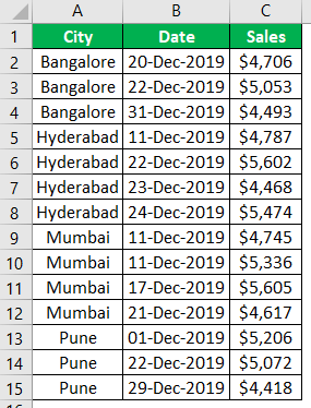
- For example, look at the below data in excel.

We need to create a city-wise sum of values in a single cell for the above data by arranging all the cities in order.
- We need to create a city-wise sum of values in a single cell for the above data by arranging all the cities in order.

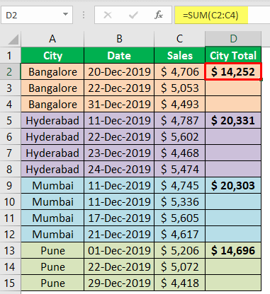
In the above image, we have an extra column as "City Total," and all the cities are sorted one after the other. Then we used the SUM function to arrive at each city's total. But the problem with the above method is we have used the SUM excel function, and for each city, there are different line items, and for each city, we need to apply the SUM function individually, so it takes a lot of time when the data is large.
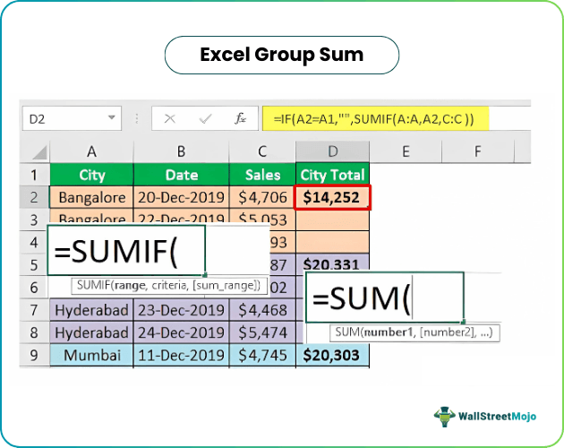
So for the city-wise total, we can use the combination formula of IF and SUMIF functions.
Example#2 - Combination Formula to Get Group-Wise Sum in Excel
Take the above data for this instance as well.
- Sort the data based on city names.

- We need the city total in the row where the city name starts. In the remaining cells, we need blank values. So, we must open the IF function now.

- We need to apply the logical test here to test whether the below cell has the same city name as the active cell, so use the logical test as below.

- If the above cell value equals the active cell value, we need a blank.

- The above logical test says if A2 is equal to A1, it returns the result as blank. Next, if this logical test is "FALSE," we need the result as the overall total of that particular city for this open SUMIF function inside the IF Excel function.

- The first argument of the SUMIF function is "Range," i.e., based on what range we would like to "SUM." So here, based on the city name, we need to sum, so we must choose the entire column of the city name.

- The next argument is "Criteria," i.e., in the selected range for which city you need to sum, giving the cell reference as A2.

- The sum range is nothing, but for the provided criteria, which column range do we want to sum, so choose the "Sales" column.

- We must close two brackets and press the "Enter" key to get the result.

- Now, apply the formula to all the cells to get the sum of sales values based on city names.

Now let me explain the result.
- In cell C2, we have the city “Bangalore” total because the logical test of IF function says if cell A2 = A1, then returns an empty cell or gives the overall total of "Bangalore" city. Since the A2 = A1 logic is not correct, it has returned the sum of the city "Bangalore."
- Now, come to the second result in cell D3. Again, we have the empty result because in this cell, A3 = A2 logical tests are "TRUE," so the result is empty.
- But when the formula reaches D5, the logical cell test is A5 = A4, so in this case, in cell A5, we have "Hyderabad," and in cell A4, we have "Bangalore," so both are different, and this time SUMIF returns the total of "Hyderabad."
- We can use this combination of IF and SUMIF to return a sum based on a group of values.
Things to Remember
- We need to sort the data based on the group we are targeting. In this example, our target was to get the total based on the city, so we sorted based on the city.
- With the PivotTable, we get the overall summary.

