Table of contents
What is Excel Formula for Grade?
The Grade system formula is nested IF in excel which verifies certain conditions and returns the particular grade if the condition is met. So, therefore, the formula that we will be using for calculating the grade must be developed so that all the conditions that we have for checking the grade slab are reviewed and returns the grade that belongs to the condition.
For example, suppose we have a data set consisting of percentage scores, and we need to calculate the grades. Then, using the easier multiple nested IF formula in Excel, we can easily figure out the complicated calculations while applying all our conditions.
- The Excel formula for grade calculation is a great way by which we can classify the data as per the nature of the characteristics of that data. Suppose if we have the data of marks obtained by the students of a class and want to know which student is better and who has achieved more marks than other students, we can calculate the grades for the marks.
- There is no inbuilt formula that can calculate the grade in Excel so we will be using the “IF” formula in excel. Since we will have multiple Grades, we will need to use the Nested IF formula excel for calculating Grades in the below cases.
How to use Excel Formula for Grade Calculation?
Example #1 – Calculating the Grade of students using Excel Formula
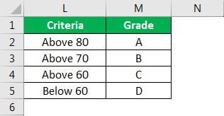
In this example of the Excel formula for the grade, we have the data of the students’ marks in their final exams, and we want to calculate the grades for the obtained marks. We have defined the criteria for grades and calculated the grades in this case. The highest marks have “A,” and the lowest have “D” grades.
Below are the steps for calculating grades of students using the excel formula –
1. First, we have to define the criteria used to return a grade for the marks scored by the student.
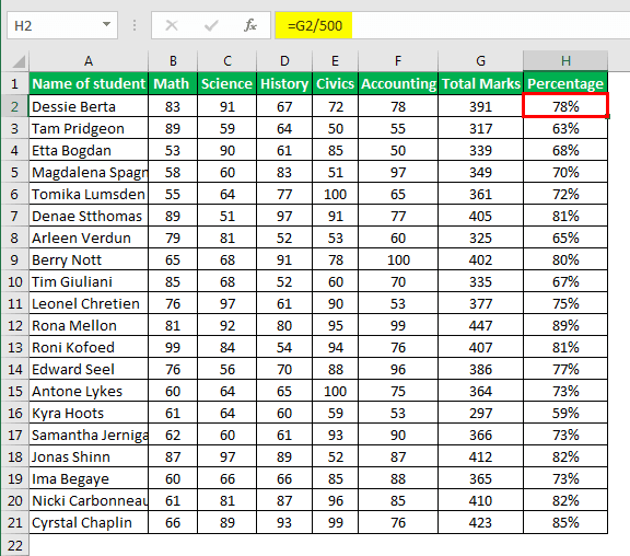
2. After the criteria are defined, we need to calculate the total marks of students and the percentage achieved by the students.
3. Now, we must use the nested IF formula:
=IF(H2>80%,”A”,IF(H2>70%,”B”,IF(H2>60%,”C””D”)))
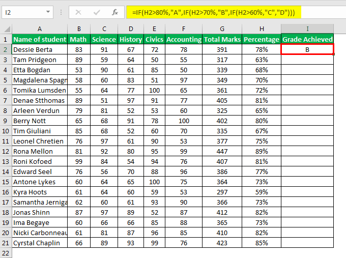
The logic that is defined in the formula is
If the percentage is more than 80 then the student falls into Grade A
=IF(H2>80%,”A”,IF(H2>70%,”B”,IF(H2>60%,”C””D”)))
If the percentage is more than 70 then the student falls into Grade B.
==IF(H2>80%,”A”,IF(H2>70%,”B”,IF(H2>60%,”C””D”)))
If the percentage is more than 60 then the student falls into Grade C.
==IF(H2>80%,”A”,IF(H2>70%,”B”,IF(H2>60%,”C””D”)))
At last, if the percentage is less than 60 then the student falls into Grade D.
==IF(H2>80%,”A”,IF(H2>70%,”B”,IF(H2>60%,”C””D”)))
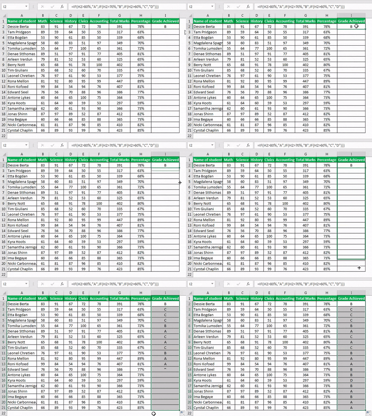
4. Now we need to drag the formula down to other cells also to calculate the grade for other students.
Example #2 – Calculating the Product Quality Grade using Excel Formula for Grade.
In this example of the Excel grade formula, we have calculated the grade of quality for fruits based on the quality score the particular veggies have obtained. The highest quality score has a good grade of A, and the lowest quality score has a D grade.
- The first step will be to set the criteria for calculating the grades.

- We have to use the nested IF formula as we have used in the above example to calculate the grade for the product quality.
The formula that we have used in this case is
=IF(B2>80%,”A”,IF(B2>70%,”B”,IF(B2>60%,”C”,”D”)))
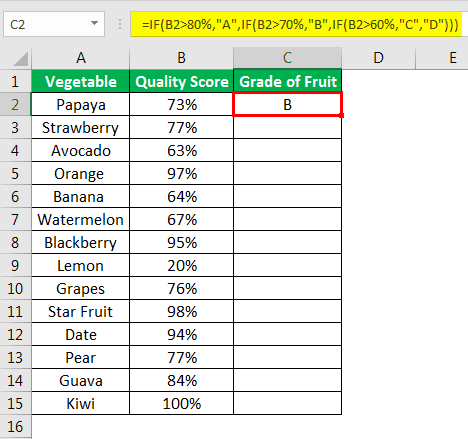
The logic that we have defined in this case is as below.
If the percentage is more than 80, than the Grade is A
=IF(B2>80%,”A”,IF(B2>70%,”B”,IF(B2>60%,”C”,”D”)))
If the percentage is more than 70, than the Grade is
=IF(B2>80%,”A”,IF(B2>70%,”B”,IF(B2>60%,”C”,”D”)))
If the percentage is more than 60, than the Grade is C.
=IF(B2>80%,”A”,IF(B2>70%,”B”,IF(B2>60%,”C”,”D”)))
At last, if the percentage is less than 60, than the Grade is D.
=IF(B2>80%,”A”,IF(B2>70%,”B”,IF(B2>60%,”C”,”D”)))
- Now we need to drag the formula down to other cells to calculate the Grade for other products also.
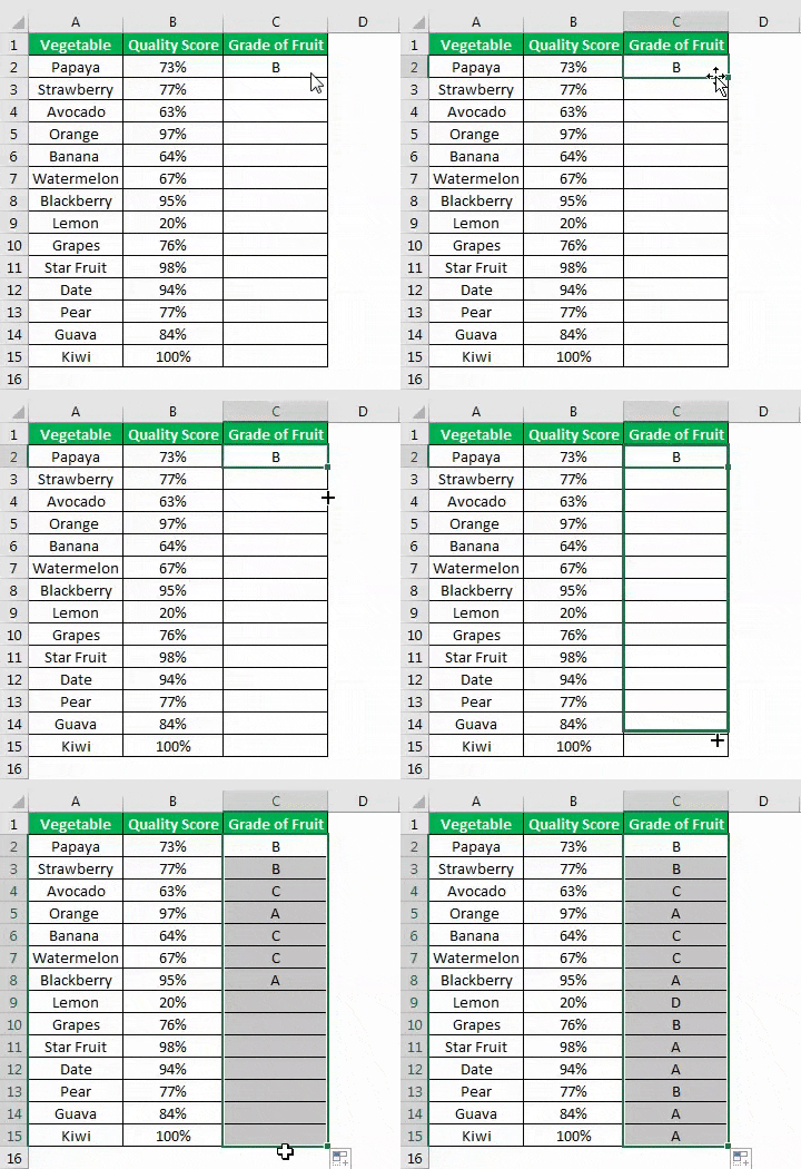
Example #3 – Calculating the Grade of quality offered by service centers.
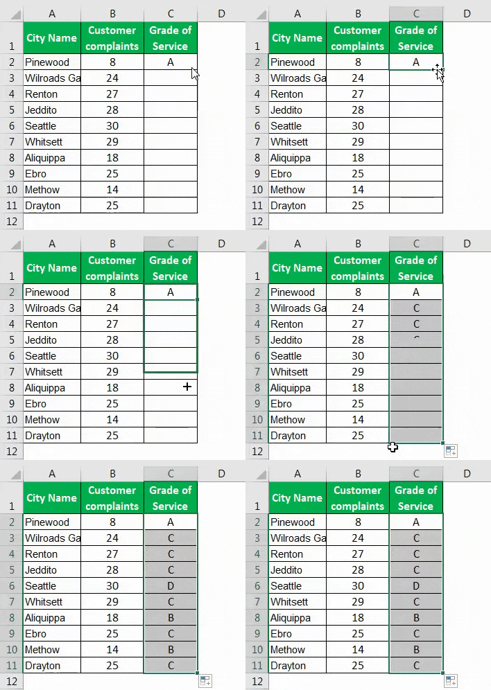
The formula that we will be using is different from the above two examples of Excel grade formulas. In this case, the criteria will be the no. of complaints lodged against the customer service center. It means the lesser the complaints, the more is the quality of service.
- The first step is to define the criteria for the grade of service.
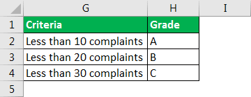
- Now, we need to use the below formula to calculate the grade. In this case, we will be using the logic of “<” instead of “>.”
The nested IF formula that we need is below.
=IF(B2<10,”A”,IF(B2<20,”B”,IF(B2<30,”C”,”D”)))
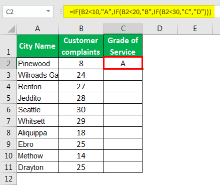
The logic is as below.
If the complaints are less than 10, than “A” grade.
=IF(B2<10,”A”,IF(B2<20,”B”,IF(B2<30,”C”,”D”)))
If the complaints are less than 20, than “B” grade.
=IF(B2<10,”A”,IF(B2<20,”B”,IF(B2<30,”C”,”D”)))
If the complaints are less than 30, than “C” grade.
=IF(B2<10,”A”,IF(B2<20,”B”,IF(B2<30,”C”,”D”)))
If the complaints do not fall in any criteria, then “D” grade.
=IF(B2<10,”A”,IF(B2<20,”B”,IF(B2<30,”C”,”D”)))
- Now we need to drag the formula down to other cells.
Things to remember about Excel Formula for Grade
- If we have a percentage instead of numbers, we also need to define % in the logical function.
- If we are calculating the grades for a case where less the number means a higher grade, then we need to use “<” instead of “>” as the operator.
- If we refer to any list as the condition that we need to ensure that the range we have referred to is locked before dragging the formula down to other cells.
- We need to remember that we need to close the formula with that many brackets equal to the numbers of “IF” we have used inside the formula. We must complete all nested IF formulas with “).”


