Table Of Contents
How to Use Excel as a Calculator?
In Excel, by default, there is no calculator button or option available in it. But, we can enable it manually from the "Options" section and then from the "Quick Access Toolbar," where we can go to the commands not available in the ribbon. There further, we will find the calculator option available. Just click on "Add" and the "OK" to add the calculator to our Excel ribbon.
I have never seen beyond Excel to do the calculations in my career. Most of the calculations are possible with Excel spreadsheets. Not only are the calculations, but they are also flexible enough to reflect the immediate results if there are any modifications to the numbers, which is the power of applying formulas.
By using formulas, we need to worry about all the steps in the calculations because formulas will capture the numbers and show immediate real-time results for us. Excel has hundreds of built-in formulas to work with some of the complex calculations. On top of this, we see the spreadsheet as a mathematics calculator to add, divide, subtract, and multiply.
This article will show you how to use Excel as a calculator.
How to Calculate in Excel Sheet?
Below are examples of how to use Excel as a calculator.
Example #1 - Use Formulas in Excel as a Calculator
As told, Excel has many of its built-in formulas, and on top of this, we can use Excel in the form of a calculator. To enter anything in the cell, we type the content in the required cell but apply the formula, and we need to start the equal sign in the cell.
Follow the below steps.
- So, to start any calculation, we need first to enter an equal sign, indicating that we are not just entering. Rather, we are entering the formula.

- Once the equal sign is entered in the cell, we can enter the formula. For example, assume that if we want to calculate the addition of two numbers, 50 and 30, we first need to enter the number we want to add.

- Once the number is entered, we need to go back to the basics of mathematics. Since we are doing the addition, we need to apply the PLUS (+) sign.

- After the addition sign (+), we must enter the second number. Then, we need to add to the first number.

- Now, press the ENTER key to get the result in cell A1.

So, 50 + 30 = 80.
It is the basic use of Excel as a calculator. Similarly, we can use cell references to the formula.
Example #2 - Use Cell References
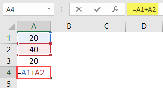
For example, look at the below values in cells A1, A2, and A3.
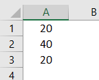
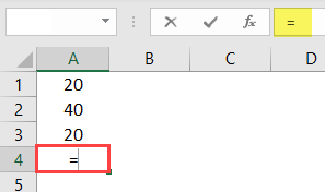
- We must open an equal sign in the A4 cell.
- Then, select cell A1 first.
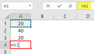
- After selecting cell A1, we need to put a plus sign and choose the A2 cell.
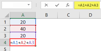
- Now, put one more plus sign and select A3 cell.
- Press the "ENTER" key to get the result in the A4 cell.
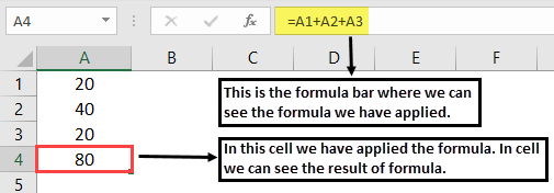
It is the result of using cell references.
Example #3 - Cell Reference Formulas are Flexible
By using cell references, we can make the formula real-time and flexible. We said cell reference formulas are flexible because if we make any changes to the formula input cells (A1, A2, A3), it will reflect the changes in the formula cell (A4).
- We will change the number in cell A2 from 40 to 50.
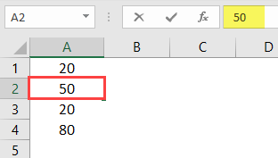
We have changed the number but have not yet pressed the "ENTER" key. If we hit the "ENTER" key, we can see the result in the A4 cell.
- The moment we press the "ENTER" key, we see the impact on cell A4.
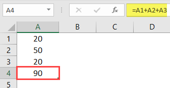
Example #4 - Formula Cell is not Value, It is the only Formula
We need to know when we use a cell reference for formulas because formula cells hold the result of the formula, not the value itself.
- Suppose we have a value of 50 in cell C2.
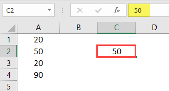
- If we copy and paste it to the next cell, we still get the value of 50 only.
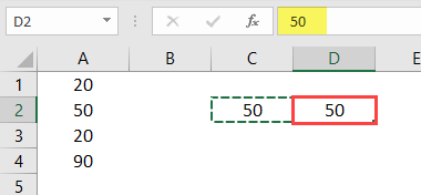
- But, now come back to cell A4.
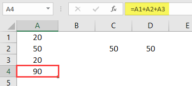
- Here we can see 90, but this is not the value but the formula. So we will copy and paste it to the next cell and see what we get.
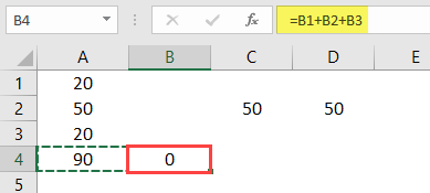
Oh oh!!! We got zero.
We got zero because cell A4 has the formula =A1 + A2 + A3. When we copy cell A4 and paste it to B4, formula-referenced cells are changed from A1 + A2 + A3 to B1 + B2 + B3.
We got zero since there are no values in the cells B1, B2, and B3. So now, we will put 60 in any of the cells in B1, B2, and B3 and see the result.
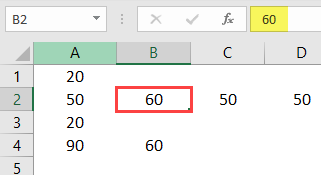
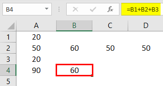
- Look here the moment we have entered 60; we got the result as 60 because cell B4 already has the cell reference of the above three cells (B1, B2, and B3).
Example #5 - Built-In Formulas are Best Suited for Excel
We have seen how to use cell references for the formulas in the above examples. But those are best suited only for the small number of data sets, for a maximum of 5 to 10 cells.
Now, look at the below data.
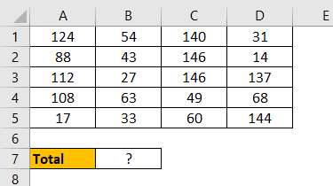
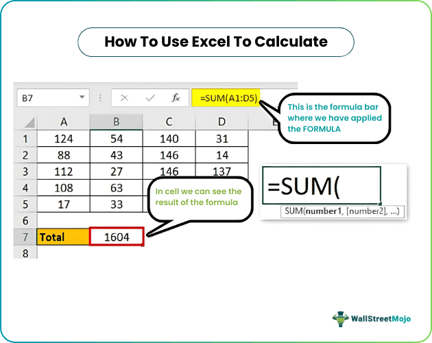
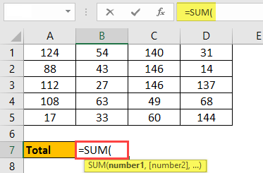
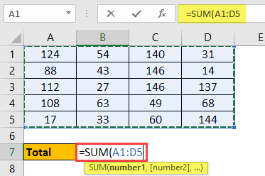
We have numbers from A1 to D5, and in the B7 cell, we need the total of these numbers. In these large data sets, we cannot give individual cell references, which takes a lot of time for us. That is where Excel’s built-in formulas come into the example.
- We should first open the SUM function in cell B7.
- Now, hold the left-click of the mouse and select the range of cells from A1 to D5.
- After that, close the bracket and press the "Enter" key.
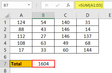
So, like this, we can use built-in formulas to work with large data sets.
This way, we can calculate in the Excel sheet.

