Excel Alternate Row Color

Publication Date :

09 Feb, 2019

Blog Author :

Edited by :

Reviewed by :

Download FREE Alternate Row Color Excel Template and Follow Along!

Alternate Row Color Excel Template.xlsx

Table Of Contents

What Is Excel Alternate Row Color?

Excel Alternate Row color, also known as banding helps users to identify data with ease. In Excel, it is simple to highlight alternate colors. We can change colors in alternate row using two methods which we will discuss in this article.

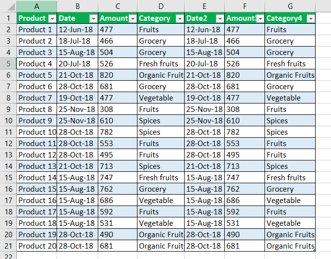
For example, consider the below table showing the names and ages of people. Now, let us highlight the alternate rows.

Excel Alternate Row Color Example - 1

Step 1: First, select the rows which we want to add color.
Step 2: Next, click on Home → Format as Table and select any table style.
Step 3: Then, the Create Table window opens up. Click My table has headers as the table in this example has headers.
Step 4: Press OK.

Excel Alternate Row Color Example - 2

Likewise, we can add alternate row color in Excel.

Key Takeaways

Excel Alternate Row color enables users to highlight alternate rows. It helps users to identify data with ease.
While using the conditional formula, we must always enter the formula in the tab. Otherwise, we will not be able to color the row.
We should use dark colors for the text to easily read the data in the Excel worksheet.
If we want to print your excel sheet, we must ensure that we use a light or decent color shade to highlight the rows to read it very easily.
We must try not to use the excess conditional formatting function in our data because it creates confusion.

How To Add Alternate Row Color In Excel?

Below mentioned are the two different methods to add color to alternative rows:

Add alternative row colors using Excel table styles
Highlight alternative rows using Excel "Conditional Formatting" option

Now, let us discuss each method in detail with an example.

#1 - Add Alternative Row Color Using Excel Table Styles

The quickest and most straightforward approach to apply row shading in Excel is by utilizing Excel table styles. Using this method, we can easily add or highlight alternative rows in excel.

#2 - Highlighting Alternate Row Color Using Excel Conditional Formatting

As the name suggests, we can use conditional formatting to highlight alternative colors in Excel.

Excel Alternate Row Color Example - Method 2

It is useful to highlight alternative rows in huge datasets.

Benefits Of Using Excel Alternate Row Colors

To improve the readability of the Excel sheet, some users shade every other row in a huge Excel sheet.
Colors can enable us to envision our information adequately by empowering us to perceive gatherings of related data by sight.
When we use the color in your spreadsheet, this theory makes the difference.
Adding shading to alternate rows or columns (which is called shading banding) can make the information in our worksheet less demanding to examine.
If any rows are inserted or deleted from the row shading, it automatically adjusts to maintain our table’s pattern.

Examples

Let us have a look at the following examples to understand both the methods in detail.

Example #1

First, we must select the data or range where we want to add the color in a row.
Then, click on the “Insert” tab on the Excel ribbon and click “Table” to choose the function.
When we click on the “Table,” the dialog box will select the range.
Click on the “OK.” Now, we will get the table with alternate row colors in Excel, as shown below:
Suppose we do not want the table with rows. We would preferably have alternate column shading just without the table usefulness. We can undoubtedly change over the table back to a standard range. We need to select any cell inside the table, right-click and choose “Convert to Range” from the setting menu.
Then, select the table or data, and go to the “Design” tab.
Next, we need to go to table style and choose the color of the table which is required and selected by us.

Example #2

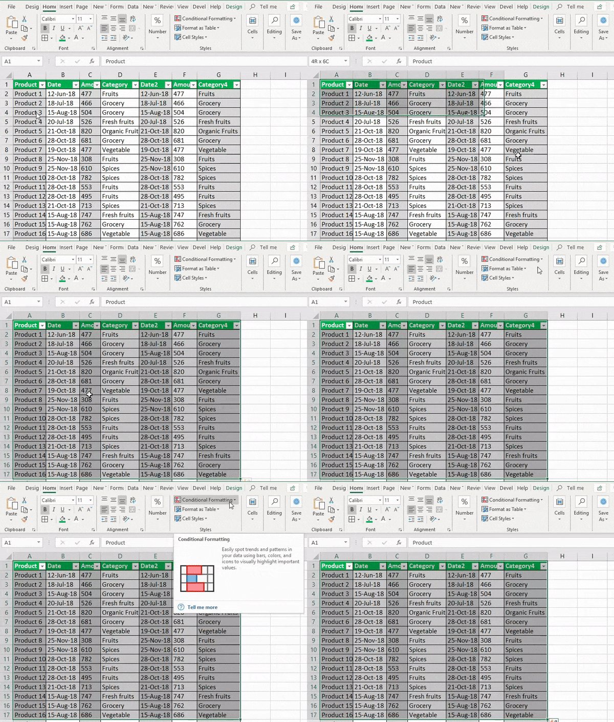
Step 1: First, we need to select the data or range in the Excel sheet.

Step 2: Go to the "Home" tab and "Styles" group, and click on conditional formatting in the Excel ribbon.

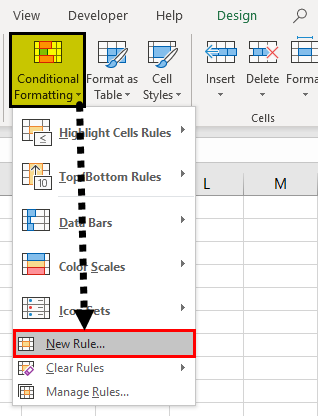
Step 3: Choose a "New Rule" from the drop-down list in excel:

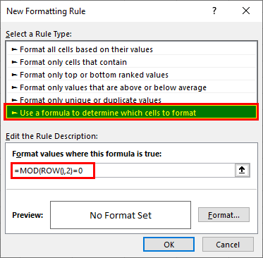
Step 4: In the “New Formatting Rule” dialog box, we must choose the option at the bottom of the dialog box, “Use a formula to determine which cells to format,” and insert the following formula in a tab to get the result.

=MOD(ROW(),2)=0

Step 5: Click the “Format” button on the right-hand side, click on the switch to the “Fill” tab, and choose the background color we want to use or required for the banded rows in the Excel sheet.

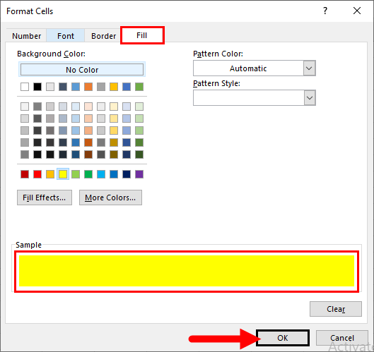
Step 6: In the dialog box, as shown above, the color we have selected will appear under the “Sample” at the bottom of the dialog box. If we are satisfied with the color, click “OK” to choose the same color, which shows in a sample.

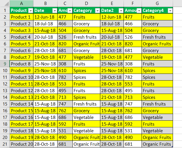
Step 7: Once we click on “OK,” it will carry us back to the “New Formatting Rule” window in the Excel sheet, and when you click “OK” again, apply the Excel color to the alternate row of the certain rows. Click “OK.” We will get the alternate row color in Excel with yellow color, as shown below.

Important Things To Note

We must always use decent colors while coloring the alternate color because the bright color cannot solve our purpose.
Highlighting alternate rows in excel is also called as banding.
We can use Excel table styles or conditional formatting.