Excel 2016 - Ribbons, Tabs and Quick Access Toolbar
Table Of Contents
Excel 2016 Ribbons
Microsoft Excel is one of the best tools ever built. It can help you perform easy tasks like calculations but also helps in performing analytical tasks, visualization, and financial modeling. This Excel training course assumes no previous knowledge of Excel, and please feel free to jump across sections if you already know a bit of Excel. This Excel 2016 tutorial is useful for people who would not get acquainted with Excel 2016 and those using older versions of Excel-like Excel 2007, Excel 2010, or Excel 2013. Most of the features and functions discussed here are common across the Excel software version. In this first post on basic Excel 2016, we will discuss the following:
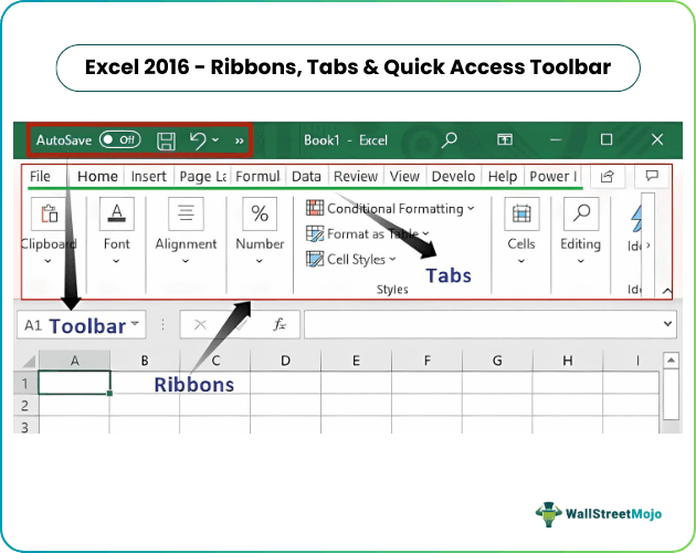
Table of contents
How to Open the Excel 2016 Software?
To open the Excel 2016 software, please go to the "Program" menu and click "Excel." If you are opening this software for the first time, worry not; we will take this Excel training step-by-step.
How to Open a blank workbook in Excel 2016
Once you open the Excel software from the "Program" menu, the first thing that you would notice is a large screen displayed as per below.
Since this is your first workbook, you will not notice any recently opened workbooks. Instead, you can choose from various options; however, this being your first tutorial, I was hoping you could open the "Blank Workbook," as shown below.
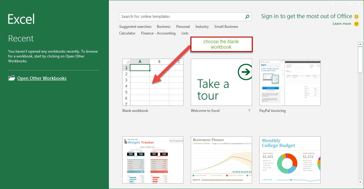
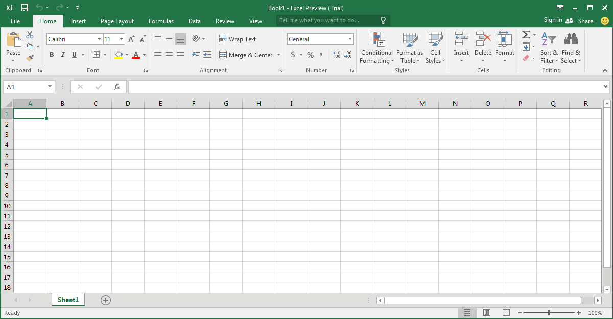
Once you click on the "Blank Workbook," you will notice the "Blank Workbook" opening in the below format.
You may also take a look at this - Head to Head Differences Between Excel and Access.
What are Ribbons in Excel
As noted in the picture below, ribbons are designed to help you quickly find the command you want to execute in Excel 2016. Ribbons are divided into logical groups called "Tabs." Each tab has its own set of unique functions to perform. For example, there are various tabs – "Home," "Insert," "Page Layout," "Formulas," "Date," "Review," and "View."

How to Collapse (Minimize) Ribbons
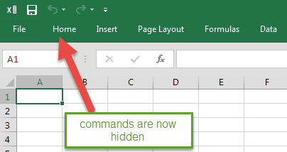
If you do not want to see the commands in the ribbons, you can always "collapse" or "minimize" ribbons.
Right-click on the "Ribbon" area, and you will see various options available here. Here, you need to choose "Collapse the Ribbon."
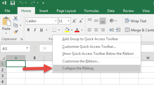
Once you choose this, the visible groups go away, and they are now hidden under the tab. But, of course, you can always click on the "Tab" to show the commands.
How to Customize Ribbons
It is often handy to customize a ribbon containing the commands you frequently use. It helps save a lot of time and effort while navigating the Excel workbook.
Follow the below-given steps to customize ribbons in Excel:
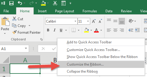
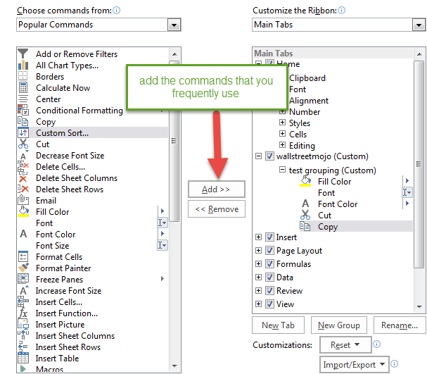
- We must first right-click on the Ribbon area to customize Excel Ribbons and choose Customize the Ribbon.
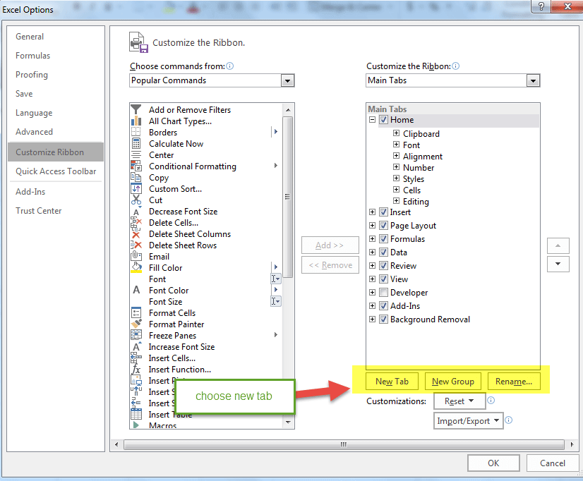
- Once the dialog box opens, click on the New Tab, as highlighted in the picture below.
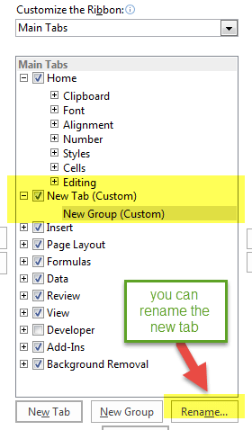
- Now, Rename the New Tab and the New Group as per your liking. We are naming the tab “wallstreetmojo” and the group name “test grouping.”
- From the left-hand side, we can select the list of commands we want to include in this New Tab.
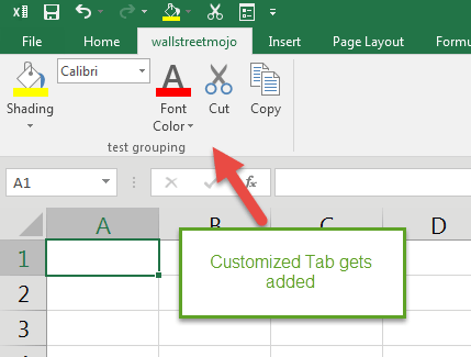
- Once we are done, we may notice that our customized tab appears in the Ribbon and the other tabs.
What is the Quick Access Toolbar
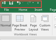
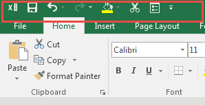
The Quick Access Toolbar is a universal toolbar that is always visible and not dependent on the tab you are working with. For example, if you are in the "Home" tab, you will see commands related to the "Home" tab, and the Quick Access Toolbar on the top executing these commands easily. Likewise, if you are in any other tab, say “Insert,” then again, you will see the same Quick Access Toolbar.
How to Customize Quick Access Toolbar
To customize the Quick Access Toolbar, we must right-click on any part of the "Ribbon," and you will see the following:

Once you click on "Customize Quick Access Toolbar," you get the dialog box from where you can select the set of commands you want to see in the Quick Access Toolbar.
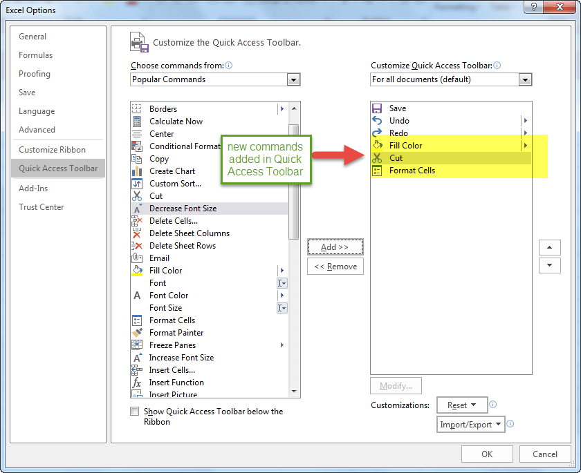 The new Quick Access Toolbar now contains the newly added commands. So as you can see, this is pretty simple.
What are the Tabs?
Tabs are nothing but various options available on the "Ribbon." These can be used for easy navigation of commands you desire to use.

Home Tab

- Clipboard - This clipboard group is primarily used for cutting, copying, and pasting. Suppose you want to transfer data from one place to another. In that case, you have two choices, COPY (preserves the data in the original location) or CUT (deletes the data from the original location). Also, there are options of Paste Special, which implies copying in the desired format. We will discuss the details of these later in the Excel tutorials. Also, Format Painter Excel, replicates the format from the original cell location to the destination cell location.
- Fonts - This font group within the "Home" tab chooses the desired "font" and "size." There are hundreds of fonts available in the drop-down, which we can use. In addition, you can change the font size from small to large, depending on your requirements. Also helpful is the feature of Bold (B), Italics (I), and Underline (U) of the fonts.
- Alignment - As the name suggests, this group is used to align tabs – "Top," "Middle," or "Bottom" alignment of text within the cell. Also, there are other standard alignment options like "Left," "Middle," and "Right" alignment. There is also an orientation option that we can use to place the text vertically or diagonally. We can use "Merge and Center" to combine more than one cell and place its content in the middle. It is a great feature to use for table formatting etc. We can also use the "Wrap text" when there is a lot of content in the cell, and we want to make all the text visible.
- Number - This group provides options for displaying number format. Various formats are available – general, accounting, percentage, comma style in excel, etc. You can also increase and decrease the decimals using this group.
- Styles - This is an interesting addition to Excel. You can have various styles for cells – Good, Bad, and Neutral. Other styles are available for data and models like calculation, check, warning, etc. In addition, you can make use of different "Titles" and "Heading" options available within "Styles." The "Format-Table" allows you to convert mundane data into an aesthetically pleasing data table quickly. Whereas "Conditional formatting" is used to format cells based on certain predefined conditions. These are very helpful in spotting patterns across an Excel sheet.
- Cells - This group is used to modify the cell – its height, width, etc. Also, you can hide and protect the cell using the "Format" feature. You can also insert and delete new cells and rows from this group.
- Editing - This group within the "Home" tab is useful for editing the data on an Excel sheet. The most prominent commands here are the Find and Replace in Excel commands. Also, you can use the sort feature to analyze your data – sort from A to Z or Z to A, or you can do a custom sort here.
Insert Tab

- Tables - This group provides an excellent way to organize the data. You can use a table to sort, filter, and format the data within the sheet. In addition, you can also use PivotTables to analyze complex data very easily. We will be using Pivot Tables in our later tutorials.
- Illustrations - This group provides a way to insert pictures, shapes, or artwork into Excel. You can insert the images directly from the computer or use the "Online Picture Option" to search for relevant pictures. In addition, shapes provide additional ready-made squares, circles, and arrows, the kind of shapes that we can use in Excel. SmartArt provides an awesome graphical representation to visually communicate data in lists, organizational charts, Venn diagram to process diagrams. The "Screenshot" can be used to quickly insert a screenshot of any program that is open on the computer.
- Apps - You can use this group to insert an existing app into Excel. You can also purchase an app from the "Store" section. For example, the "Bing Maps" app allows you to use the location data from a given column and plot it on "Bing Maps." Also, a new feature called "People Data" allows you to transform boring data into an exciting one.
- Charts - This is one of the most useful features in Excel. It helps you visualize the data in a graphical format. The "Recommended" charts allow Excel to develop the best graphic combination. In addition, you can make graphs on your own, and Excel provides various options like pie-chart, line charts, Column Chart in Excel, Bubble Chart k in Excel, combo chart in excel, Radar Chart in Excel, and Pivot Charts in Excel.
- Sparklines - Sparklines are tiny charts made on the number of data and can be displayed with these cells. Different options are available for sparklines like "Line Sparkline," "Column Sparkline," and "Win/Loss Sparkline." We will discuss this in detail in later posts.
- Filters - There are two types of filters available: "Slicer" allows you to filter the data visually and can be used to filter tables, PivotTables data, etc. The "Timeline" filter allows you to filter the dates interactively.
- Hyperlink - It is a great tool to provide hyperlinks from the Excel sheet to an external URL or files. We can also use hyperlinks to create a navigation structure with the Excel sheet that is easy to use.
- Text - This group is used to text in the desired format. For example, you can use this group to have the header and footer. In addition, "WordArt" allows you to use different styling for text. You can also create your signature using the "Signature" line feature.
- Symbols - This primarily consists of two parts – a) Equation – it allows you to write mathematical equations that we cannot ordinarily write in an Excel sheet. 2) Symbols - They are special characters or symbols that we may want to insert into the Excel sheet for better representation.
Page Layout Tab
 Themes - Themes allow you to change Excel's style and visual look. You can choose various types available from the "Menu." You can also customize the Excel workbook's colors, fonts, and effects.
- Page Setup - This is an important group primarily used to print printing an excel sheet. You can choose margins for the print. In addition, you can select your printing orientation from "Portrait" to "Landscape." Also, you can choose the size of paper like "A3," "A4," "Letterhead," etc. The print area allows you to see the print area within the excel sheet and helps make the necessary adjustments. We can also add a break where we want the next page to begin in the printed copy. Also, you can add a background to the worksheet to create a style. "Print Titles" is like a header and footer in excel that we want to be repeated on each printed copy of the Excel sheet.
- Scale to Fit - This option is used to stretch or shrink the printout of the page to a percentage of the original size. You can also shrink the width and height to fit a certain number of pages.
- Sheet Options - The "Sheet Options" is another useful feature for printing. We can check the print gridlines option if we want to print the grid. If we print the row and column numbers in the Excel sheet, we can also do the same using this feature.
- Arrange - Here, we have different options for objects inserted in Excel like "Bring Forward," "Send Backward," "Selection Pane," "Align," "Group Objects," and "Rotate."
Formulas Tab

- Function Library - This is a very functional group containing all the formulas used in Excel. This group is subdivided into important functions like "Financial Functions," "Logical Functions," "Date & Timing," "Lookup & References," "Maths and Trigonometry," and other functions. One can also use the "Insert'' function capabilities to insert the function in a cell.
- Defined Names - This feature is fairly advanced but useful. We can use it to name the cell, and these named cells can be called from any part of the worksheet without working about their exact locations.
- Formula Auditing - This feature audits the flow of formulas and their linkages. It can trace the precedents (origin of data set) and show which dataset depends on this. We can also use the "Show Formula" to debug errors in the formula. The Watch window in excel is also useful to keep a tab on their values as you update other formulas and datasets in the Excel sheet.
- Calculations - By default, the option selected for calculation is automatic. However, one can also change this option to manual.
Data Tab

- Get External Data - This option is used to import external data from various sources like "Access," "Web," "Text," "SQL Server," "XML," etc.
- Power Query - This advanced feature combines data from multiple sources and presents it in the desired format.
- Connections - This feature is used to refresh the Excel sheet when the data in the current Excel sheet is coming from outside sources. You can also display the external links and edit those links from this feature.
- Sort & Filter - We can use this feature to sort the data from A to Z or Z to Z, and also, you can filter the data using the drop-down menus. Also, one can choose advanced features to filter using complex criteria.
- Data Tools - This is another very useful group for advanced excel users. One can create various scenario analyses using What-If analysis – Data Tables, Goal Seek in Excel, and Scenario Manager. Also, one can convert Text to Column, remove duplicates and consolidate from this group.
- Forecast - We can use this "Forecast" function to predict the values based on historical values.
- Outline - One can easily present the data intuitively using the "Group" and "Ungroup" options from this.
Review Tab

- Proofing - It is an interesting feature in Excel that allows you to run spell checks in the excel. In addition to spell checks, one can also use a thesaurus if you find the right word. A research button also helps you navigate the encyclopedia, dictionaries, etc., to perform tasks better.
- Language - If you need to translate your excel sheet from English to any other language, you can use this feature.
- Comments - Comments are very helpful when you want to write an additional note for important cells. It helps the user understand clearly the reasons behind your calculations etc.
- Changes - If you want to keep track of the changes that are made, you can use the Track Changes option. Also, you can protect the worksheet or the workbook using a password from this option.
View Tab

- Workbook Views - You can choose the viewing option of the Excel sheet from this group. You can view the Excel sheet in the normal default view, select the "Page Break" view, "Page Layout" view, or any other custom view.
- Show - We can use this feature to show or not show formula bars, grid lines, or heading in the Excel sheet.
- Zoom - Sometimes, an Excel sheet may contain a lot of data, and you may want to change zoom in or zoom out desired areas of the Excel sheet.
- Window - The new window is a helpful feature that allows users to open the second window and work on both simultaneously. Also, freeze panes are another useful feature that helps to freeze particular rows and columns such that they are always visible even when one scrolls to extreme positions. You can also split the worksheet into two parts for separate navigation.
- Macros - This is again a fairly advanced feature, and you can use this feature to automate certain tasks in Excel Sheets. "Macros" are nothing but a recorder of actions taken in Excel, and they can execute the same steps again if required.
Recommended Articles
What next?
If you learned something new or enjoyed this post, please comment below. Let me know what you think. Many thanks, and take care. Happy Learning!
