Table Of Contents
What Is ERROR.TYPE Function In Excel?
The ERROR.TYPE function in Excel is an inbuilt Information function. It accepts an error value and returns a number corresponding to it as the error type. But if the input is not an error value or an error value of an unsupported type, the function returns the #N/A error.
Users can use the ERROR.TYPE() with the IF() to display a customized message for a specific error value when working with financial data.
For example, the following dataset contains two sets of values in columns A and B.
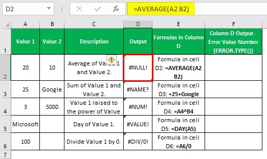
The source dataset shows the formulas applied in column D based on the descriptions specified in column C. However, the outputs in column D are error values.
The aim is to determine the number corresponding to each column D error value and display the output in column F.
Then, we can use the Excel ERROR.TYPE function in each target cell to achieve the required output.
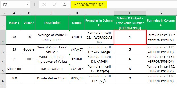
In the above Excel ERROR.TYPE function example, the ERROR.TYPE() in each target cell accepts the cell reference to the error value in the corresponding row. It then returns the number matching the specified error value.
Table of contents
- The ERROR.TYPE functionin Excel accepts an error value to return its corresponding number, code, or index as the error type.
- Users can use the ERROR.TYPE Excel function to check the type of error a formula returns in a cell. So, the function helps users to categorize error values and resolve them in an order.
- The ERROR.TYPE Excel function accepts one mandatory argument value, error_val.
- While we can use the ERROR.TYPE Excel function as a standalone function, using it with other inbuilt functions, such as IF and IFERROR, helps achieve practical results.
Syntax
The ERROR.TYPE function syntax is as follows:

Where,
- error_val: The error value whose corresponding or identifying number we aim to determine. It is a mandatory argument.
The ERROR.TYPE() argument can be an error value or the reference to the cell that has the formula we aim to test for error and obtain the corresponding number.
Furthermore, the ERROR.TYPE function for Mac is available, just like in all Excel versions from 2003.
Errors And Codes
The following table lists the errors we typically face while working with Excel data and their codes or indices, which we obtain as the ERROR.TYPE function output.
| Error_val | ERROR.TYPE() Output |
|---|---|
| #NULL! | 1 |
| #DIV/0! | 2 |
| #VALUE! | 3 |
| #REF! | 4 |
| #NAME? | 5 |
| #NUM! | 6 |
| #N/A | 7 |
| #GETTING_DATA | 8 |
| Any Non-error Value | #N/A |
Please note that the #GETTING_DATA error is a temporary error that we may face while calculating massive Excel data. We will see this error when the previous calculation is under process, and it disappears once the evaluation is complete.
The error codes or numbers help us categorize the errors in an order and resolve them accordingly.
How To Use ERROR.TYPE Function In Excel?
We can utilize the ERROR.TYPE function in two ways:
- Access the function from the Excel ribbon.
- Enter the function into the worksheet manually.
Method #1 - Access The Function From The Excel Ribbon
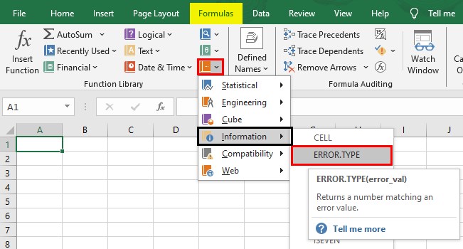
Choose a cell for output - The Formulas tab - The More Functions down arrow - The Information function group right arrow - ERROR.TYPE.
The Function Arguments window appears. Enter the argument in the Error_val field.
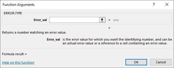
Finally, clicking OK in the Function Arguments window will show the ERROR.TYPE() output in the target cell.
Method #2 - Enter The Function Into The Worksheet Manually
- Select a cell to show the output.
- Type =ERROR.TYPE( in the cell.
- Enter the argument as a value or cell reference and close the brackets.
- Press Enter to view the ERROR.TYPE() output as the required error index or number.
Please note that the above methods will work for ERROR.TYPE function for Mac, like in Excel 2003 version and above.
Examples
Check out the following ERROR.TYPE function examples to use it effectively.
Example #1 - Identifying A #DIV/0! Error
The following dataset contains two sets of data.
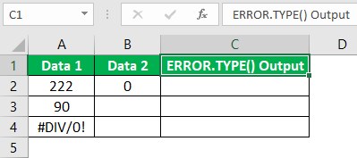
The aim is to find the error code of the error value obtained when dividing the first data by the second in row 2, dividing the first data by 0 in row 3 and for the error value in row 4. Assume the target cells are in column C.
Then, here is how to use the ERROR.TYPE function in the target cells to achieve the required output.
Step 1: Choose cell C2. Next, enter the ERROR.TYPE() and press Enter.
=ERROR.TYPE(A2/B2)
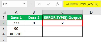
Step 2: Choose cell C3. Enter the ERROR.TYPE() and press Enter.
=ERROR.TYPE(A3/0)
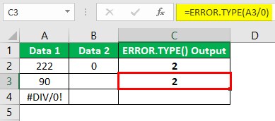
Step 3: Choose cell C4. After that, enter the ERROR.TYPE() and press Enter.
=ERROR.TYPE(A4)
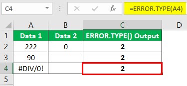
In the above example, we supply a formula returning the #DIV/0! Excel error value or cell reference to the #DIV/0! error value as the argument value to the ERROR.TYPE(). So, the function returns the corresponding error code as the output, 2, in each case, helping us to identify the error value.
Example #2 - Identifying A #NAME? Error
The following image shows a dataset containing a list of students and their test scores in three subjects.
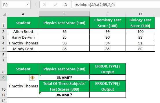
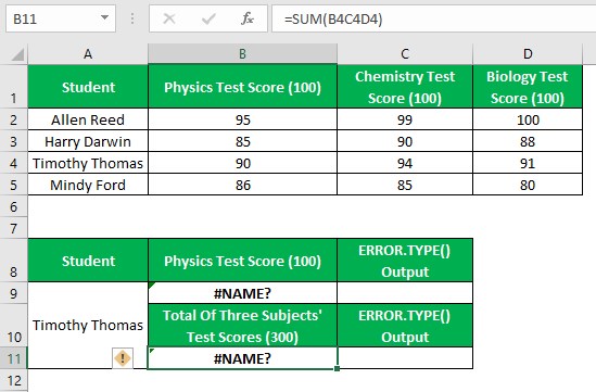
Furthermore, we apply the Excel VLOOKUP function and SUM function in cells B9 and B11. It is to determine the Physics test score and the total of the three subjects’ test scores of the specified student based on the source dataset.
However, the functions return error values. Thus, here is how to identify the #NAME? error value and display the output. Assume the target cells are C9 and C11.
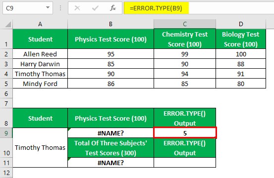
Step 1: Choose cell C9. Next, enter the ERROR.TYPE function and press Enter.
=ERROR.TYPE(B9)
Step 2: Choose cell C11. Enter the ERROR.TYPE function and press Enter.
=ERROR.TYPE(B11)
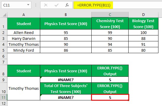
In the case of cells B9 and B11, the VLOOKUP() name and the input supplied to the SUM() are incorrect, leading to the functions returning the #NAME? error value.
So, we supply the reference to the cells B9 and B11, containing the formulas, as the inputs to the ERROR.TYPE() in the target cells C9 and C11. The function thus returns the corresponding error code, 5, in each target cell, which helps identify the #NAME? error value in the specified cells.
Example #3 - Using ERROR.TYPE With IFERROR
The following dataset contains two sets of inputs.
We add the two inputs in each row and display the output values in column C cells.
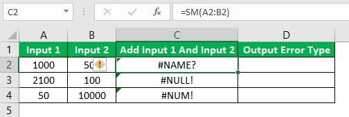

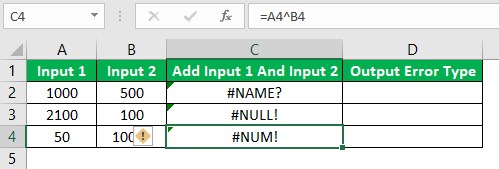
However, the output values in column C cells are error values. While in cell C2, the SUM() name is incorrect, the input supplied to the SUM() in cell C3 is incorrect. On the other hand, the addition symbol entered in cell C4 is incorrect, leading to the formula returning an error value.
Consider the task to identify the error type in each row in the form of codes or numbers and display the output in column D.
Then, we can use the ERROR.TYPE function with the Excel IFERROR function in each target cell to obtain the required error index.
Step 1: Choose cell D2. Next, enter the IFERROR() containing the ERROR.TYPE() and press Enter.
=IFERROR(C2,"The Error Type Is: "&ERROR.TYPE(C2))

Step 2: Using the Excel fill handle, update the formula in the remaining target cells.

First, the IFERROR() checks if the reference to the cell, supplied as the first argument value, contains an error value. Since the cell referred to contains an error value, the ERROR.TYPE() accepts the same cell reference to return the corresponding error code.
Thus, the formula concatenates the specified text with the ERROR.TYPE() output to return the required error type as the IFERROR() in each target cell.
Example #4 - Using ERROR.TYPE Function With IF Function
The following dataset shows input employee details.
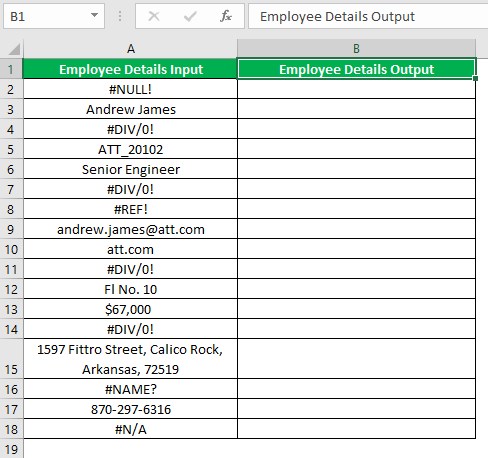
The task is to show the valid employee details in column B and leave the cell in column B empty if the corresponding cell in column A contains an error value.
But, if the column A cell contains the #DIV/0! error value, the corresponding column B cell must show the message, “Divide By Zero Error”.
Then, we can use the troubleshoot ERROR.TYPE function with the Excel IF function and ISNA function in each target cell to obtain the desired outcome.
Step 1: Choose cell B2, enter the following formula, and press Enter.
=IF(ISNA(ERROR.TYPE(A2)),A2,IF(ERROR.TYPE(A2)=2,"Divide By Zero Error",""))
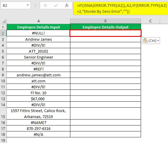
Step 2: Using the fill handle, update the formula in the remaining target cells.
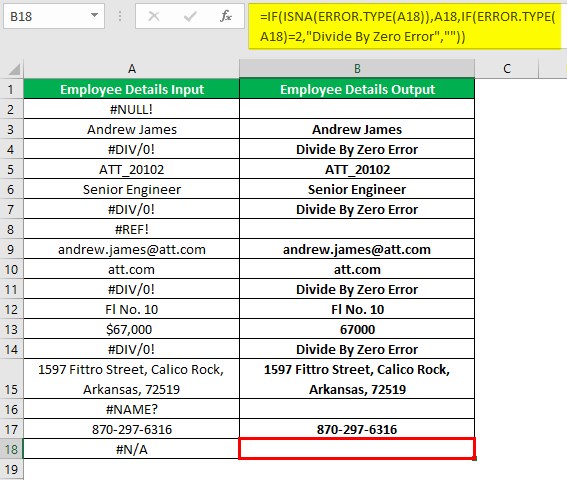
Let us check the cell B18 formula to determine the logic.
First, the ERROR.TYPE() in the ISNA() accepts the reference to cell A18, containing the source data, the #N/A error value, and returns the corresponding error type, 7.
Next, the ISNA() accepts the ERROR.TYPE() output, 7, as the input. Since the ISNA() input value is not the #N/A error value, the function output is FALSE.
So, the FALSE value in the formula, which is the IF(), gets executed.
Next, the ERROR.TYPE() gets executed as the IF() condition. The function accepts the reference to cell A18, containing the #N/A error value, and returns the corresponding error type, 7.
Next, the ERROR.TYPE() output of 7 is not equal to 2. So, the IF condition does not hold.
So, the IF() returns the FALSE value, a blank, as the formula output.
Thus, in this way, we can use the troubleshoot ERROR.TYPE function with the IF() to identify the error type and display the required output based on the specific error type.
Important Things To Note
- Ensure to supply an error value or a formula returning an error value as the argument value to the ERROR.TYPE function whose type the function recognizes. Otherwise, the function output will be the #N/A error.
- The ERROR.TYPE Excel function can return 1 to 8 error types based on the input error value or formula returning an error value.
Frequently Asked Questions (FAQs)
We can fix the #VALUE! error using ERROR.TYPE function using the following steps explained with an example.
The following image shows a dataset containing two sets of values.
We use the two sets of values to apply the required formulas in column D based on the descriptions in column C. However, the output in column D cells is the #VALUE! error due to various reasons.


Here is how to fix the #VALUE! error using the ERROR.TYPE() within the IF() in each target cell. Assume column E cells as the target cells.
Step 1: Choose cell E2, enter the following formula, and press Enter.
=IF(ERROR.TYPE(D2)=3,"Check data type for the formula.",D2)
Step 2: Using the fill handle, implement the formula in the remaining target cells.
Let us check the cell E4 formula to understand how it works.
First, the ERROR.TYPE() executes as the IF() condition. It accepts the reference to cell D4, containing the #VALUE! error value, and returns the corresponding error type as a number value, 3. Next, the ERROR.TYPE() output equals 3. So, the IF condition holds, leading to the IF() returning the TRUE value, the “Check data type for the formula.” message, as the function output.
Thus, in this way, we can fix the #VALUE! error value using the ERROR.TYPE().
The common mistakes users make while using ERROR.TYPE function are as follows:
• The users may not use the ERROR.TYPE() with an error value.
• The users sometimes use the ERROR.TYPE() with an error type that the function does not support.
Your ERROR.TYPE function is not working due to the following reasons:
• The function syntax is incorrect or contains a typo error.
• The cell reference, supplied as the ERROR.TYPE() argument value does not contain an error value of a recognized type.
Download Template
This article must be helpful to understand the ERROR.TYPE Function, with its formula and examples. You can download the template here to use it instantly.
Recommended Articles
This has been a guide to What Is ERROR.TYPE Function in Excel. Here we learn the ERROR.TYPE Excel function syntax & how to use it with examples & points to remember. You can learn more from the following articles –
