Equations In Excel

Publication Date :

24 Dec, 2018

Blog Author :

Edited by :

Reviewed by :

Download FREE Equations Excel Template and Follow Along!

Equations Excel Template.xlsx

Table Of Contents

What Do You Mean By Equations In Excel?

Equations in Excel are none other than our formulas which we type in a cell. Therefore, we must start with an equal sign (=), which Excel recognizes as a calculation to write an equation. Then we use variables connected with some operators. Depending upon the operators we get results, an equation can be both or nonlinear.

For example, Excel uses both cell references and basic operators to make an equation.

Equations In Excel

Key Takeaways

Equations in Excel help us understand the different ways to write a formula,
By manually creating a formula by entering in the cell, and taking the cell values or cell references.
By using the inbuilt functions from the “Function Library” group in the “Formulas” tab.
When we lock the Excel Equations, it prevents the user from editing, modifying, or deleting the formulas while multiple users work on a shared workbook.
When we hide the Excel Equations, the formula doesn’t display in the formula bar, i.e., it is hidden from the users who work on the shared workbook.

Explanation

Playvolume00:00/01:00TruvidfullScreen

In an Excel Equation, we use two things:

Cell References.
Operators.

Cell references are cells like A1, B1, or range of cells A1:A3 and so on, whereas operators are the basic operators such as + for sum, – for subtraction, * for multiplication, and so on.

Excel can execute formulas such as addition and subtraction like a calculator. However, one of the most useful features of MS Excel is the ability to calculate using a cell address to represent a value in a cell. It is the basic definition of the cell reference.

How To Use Equations In Excel?

We can use the Equations in Excel keeping the following three things in mind, namely:

Every equation starts with an Equals sign (=).
Excel uses cell addresses or cell values.
Operators are used to perform an equation.

Examples

We will consider examples for Equations in Excel.

Example #1

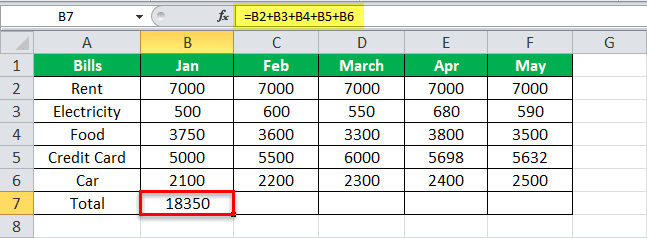
The below image has my monthly budget for five months. The budget includes rent, food, electricity, credit card, and car data.

We will create an equation for the sum or addition of the bills for each month.

Bills	Jan	Feb	March	Apr	May
Rent	7000	7000	7000	7000	7000
Electricity	500	600	550	680	590
Food	3750	3600	3300	3800	3500
Credit Card	5000	5500	6000	5698	5632
Car	2100	2200	2300	2400	2500
Total

The steps to create an equation for the sum or addition of bills for each month are,

In cell B7, we must start typing an equal sign and add each cell reference from B1 to B6 with a + operator.
When we press enter, we get the total spending done in January.

In the above two steps, we used cell references and an operator + for addition, and we created the equation as =B2+B3+B4+B5+B6, which gave us our result.

Alternatively, an inbuilt function in Excel gives us the same result, but it saves us the time of giving each cell reference one at a time.

The steps to use an inbuilt function for the sum or addition of bills for each month are,

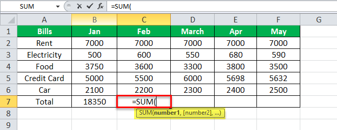
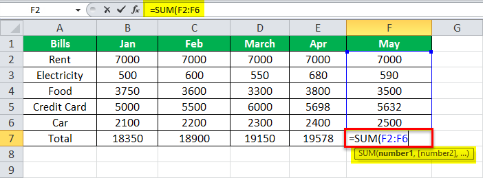
Step #1 - In cell C7, start typing an “equals to” sign, type sum, then select the “SUM” function. As a result, it opens an inbuilt sum function for us, as shown below.

Step #2 – Now, we must select the range of cells from C2 to C6, and press the “Enter” key.

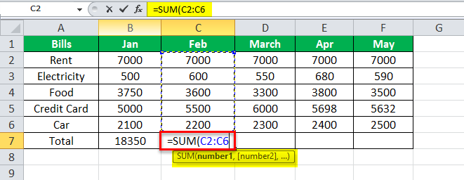
It may also give the total money spent in February.

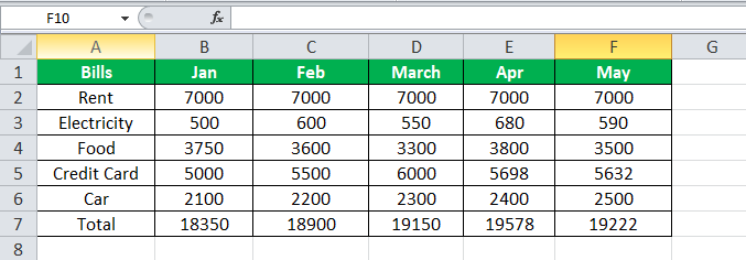
Step #3 - We may repeat the same process for March and April and get the total money paid for the respective months.

The final output shown below in Row 7 displays the money spent on all the months.

Example #2

We want Excel to inform us if the money spent was high or average. For example, if the amount paid for five months is above $10,000, it should show as “High” or “Average”. The operators used in this type of equation are “IF Statements”.

The steps to find the SUM along with the IF conditions are,

Step #1 - First, we must total the money spent on each bill. In cell G2, we will create an equation for adding the money spent on rent for five months. We start by typing an Equals sign, typing Sum, and select the “SUM” function, as shown below.

Step #2 - Select the cell references B2 to F6 and press the “Enter” key.

Step #3 - We repeat the same addition equation for every bill.

Step #4 - Now, in cell H2, type an Equals sign, type “IF”, then select the “IF” function, as shown below.

Step #5 - To better understand the IF equation, click “fx” in the function address bar.

Consequently, a dialog box pops up, as shown below.

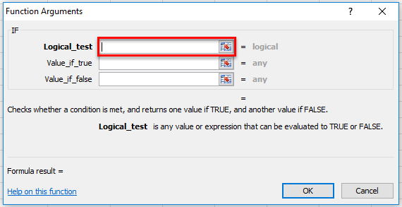
Step #6 - In the logical test, we must insert our logic: the total of bills is greater than $10,000. Then, select range G2 to G6 and insert the greater than operator “>”, and type $10,000.

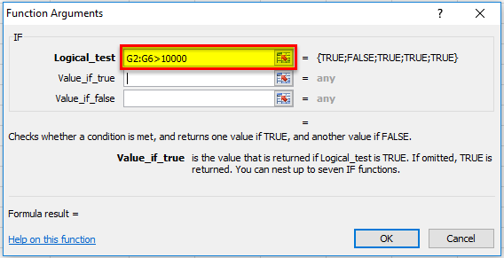
Step #7 - If the value is true, it means the total is greater than $10,000, and we want it to show as “High” or “Average”.

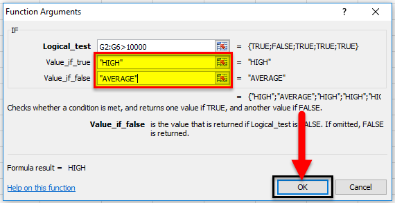
Step #8 - As we provide Excel values in the string, we must start and end it with inverted commas. After that, click “OK.”

Step #9 - Then, drag the formula to cell H6, and we may have our final output.

In the above example, we have used cell references and IF statements as an operator to make an equation.

Important Things To Note

We must always remember to start an equation with an equal sign.
Creating an equation with cell reference is useful because we can update our data without having to rewrite the formula.
Excel may not always tell us if our equation is wrong or not. So, it is up to us to check all of our equations.