Table Of Contents
Editing Drop-Down List in Excel
Before we edit drop-down lists in Excel, we must know what a list in Excel is. In simplified terms, lists in Excel are columns in Excel. But in columns, we do not have any drop-downs. Instead, we enter values manually or paste the data from any other source. But, if we are creating surveys or asking any other user to enter data and want to give some specific options to choose from, drop-downs in Excel come in handy.
As explained above, drop-downs in Excel help guide a user to manually enter values in a cell with some specific values to choose from. Like in surveys, if there is a question about the gender of a person, if we ask every user to enter values for that question, then data will not be in order. Some people may write answers in uppercase, some in lowercase, or some may make some spelling mistakes. But if we give users two values to choose from, either male or female, our data would be in the exact order we want. It is done by creating a drop-down lists in excel.
There are various ways of editing drop-down lists in Excel. They are:
- Giving drop-down values manually and using data validation.
- Offering drop-down ranges and using data validation.
- Creating a table and using data validation.
The data validation is an option under the "Data" tab in the "Data Tools" section.
How to Edit Drop-Down List in Excel?
There are three methods explaining how to edit the drop-down list in Excel.
Let us learn to make drop-down lists with some examples and learn every process to edit the drop-down list in Excel.
Example #1 - Giving Drop Down Values Manually and Using Data Validation.
We need to have the drop-down values ready to enter for the step. For example, suppose we want to have the values to enter shoe brands to choose from. Now, we need to select a cell where we will insert the drop-down.
- In cell B2, we will enter our drop-down list.

- Next, click on "Data Validation" in the "Data" tab under the "Data Tools" section.

- Again, click on "Data Validation" in Excel, and a dialog box appears.

- In "Settings," under the "Allow," select "List."
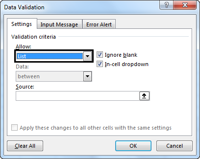
- In the "Source" section, we must manually enter the values for the drop-down options.

- When we click on the "OK," we may have our drop-down created.

The above method is the easiest way to make and edit a drop-down list in Excel. But, if we have to enter more values for the choice of shoes, we have to redo the whole process.
Example #2 - Giving Drop Down Ranges and Using Data Validation.
For example, I am a teacher, and I want a response from my students whether they have completed their projects or not. Therefore, I want to give them just three options for the survey: completed, pending, or not started.
Yes, I can use the above process, but the user can change it as they can go to the "Data Validation" tab and change the values. In this process, we select a range of values and hide the columns so that the other user cannot edit the validation or the dropdown.
- We must copy values for drop-downs or write them down in a list or column.
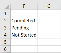
- In the cell we want to enter the validation, we will select the cell, cell B2.
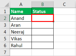
- Under the "Data" tab in the "Data Tools" section, we need to next click on "Data Validation."

- Again, we need to click on "Data Validation." As a result, a wizard box appears.
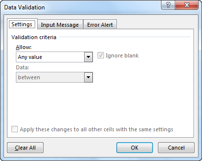
- In the settings, under "Allow," click on "List."

- In the "Source" tab, we must select the range of data for the drop-down list.
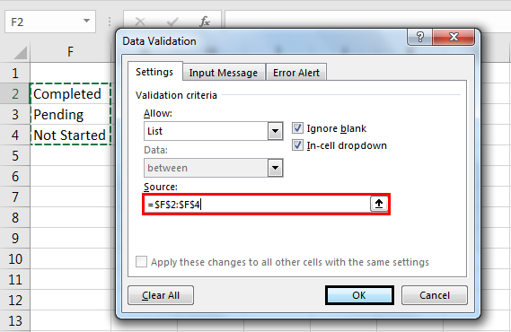
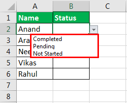
- When we click on "OK," we may have a drop-down in cell B2.
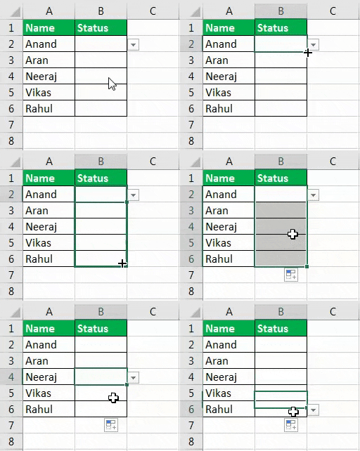
- After that, we need to copy the validation to all the cells (up to cell B6). Then, finally, we have to drop down a list of all the cells we want.
Even if we hide our cell range, which was the drop-down source, any user cannot edit the validation. The above process also has the same disadvantage as the first example. If we have to insert another option of "Half Completed," we have to redo the process again. I have to insert a new alternative to the source and new validation.
Example #3 - Creating a Data Table and Using Data Validation.
We will create a data table and use data validation as before in this method. But it will explain the benefit of using this method later on. For example, I have a restaurant and have some dishes to select for customers. So I have inserted the data in the column below.
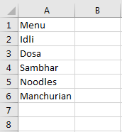
- The first step is to create a table. Then, we must select the data, and in the "Insert" tab, click on "Tables."
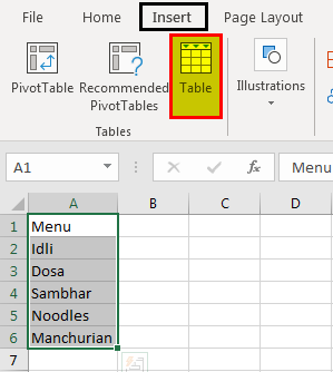
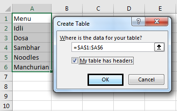
- The following window will open, and when we click "OK," we have created our table in column A.
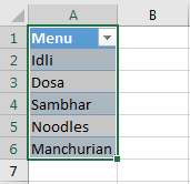
- Let us name this table "Restaurant." In the left corner, we can see an option to rename the table.
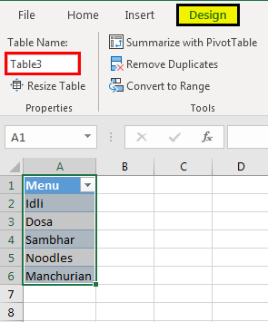
- Rename the table as "Restaurant."
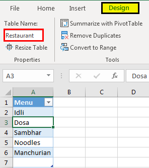
- Now, we must select the cell where we want to insert the drop-down list.
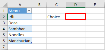
- Under the "Data" tab, now we must click on "Data Validation."

- In the "Allow" tab, select "List."

- Now in "Source," type as shown in the dialog box below.
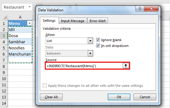
- When we click on "OK," we can see that a drop-down has been inserted into the data.
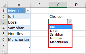
- If we have another menu to add, suppose "Soups."
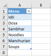
- We can see that the new entry in the "Menu" tab is also displayed in our drop-down.
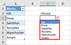
The above process has solved our problem: a new entry has to be created, and we must make drop-downs again.
Explanation of Edit Drop-Down List in Excel
I have already explained above why we need drop-down lists in our data. It helps guide a user to manually enter values in a cell with specific values to choose from.
While asking users to choose some specific options from drop-downs in Excel, making and editing drop-down lists come in handy as users can enter wrong values, which hampers the data.
Things to Remember While Editing Drop-Down List in Excel
- If we enter drop-down values manually or set ranges, any newer entry needs to be inserted with a new drop-down list.
- In tables, we can insert a new entry, updated in the dropdown.
- To view or edit the drop-down list, we need to click on the cell.

