Table Of Contents
What is DSUM in Excel?
The function DSUM in Excel is also known as the DATABASE SUM function in Excel, which is used to calculate the sum of the given database based on a certain field and provided criteria. This function takes three arguments as inputs: the range for the database, an argument for the field, and a condition, and then it calculates the sum for it.
For example, suppose we have a dataset with an order number greater than 100 and the quantity equal to or greater than 10. We need to determine the total number of records. In such a scenario, using the DSUM function in Excel, we can calculate the sum of such orders.
Syntax
Below is the DSUM Formula in Excel:

- Database: It is simply the data table along with headers.
- Field: The column you would like to sum in the data table. i.e., column header.
- Criteria: List of criteria in the cells containing the conditions specified by the user.
How to Use the DSUM Function in Excel?
The below image shows the sale of stationery items, and we have some requirements to calculate. We have five different situations to calculate the revenue. Each situation is not a different situation but conditions that we need to implement.
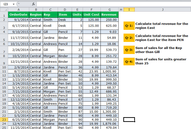
The DSUM is a criteria-based function that can return the value based on your criteria. It will give you the sum of the column based on multiple requirements. For example, total sales for the salesperson in the region west for the product desk. So it is a bit of a SUMIFS kind of function. Based on certain criteria, it will return the value.
How does DSUM Work?
The word database is not a stranger to excelling users. In Excel for the database, we use the word range of cells or cells or tables, etc. As we mentioned earlier in the article, the DSUM is a database function based on the criteria we express in a range of cells following the same database or table structure. We can give criteria to each column by mentioning it as a header and the given criteria under it.
If you already know how SUMIF and SUMIFS work, then DSUM should not be a complex thing to understand.
Let us learn ahead to get an idea about the functionality of the DSUM function.
Practical DSUM Examples
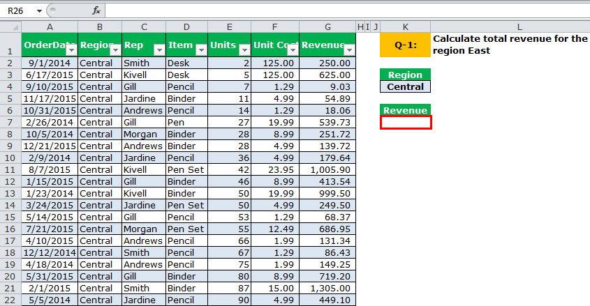
Look at the below image where we have sales data from A1 to G38. Then, answer all the questions from the below table.
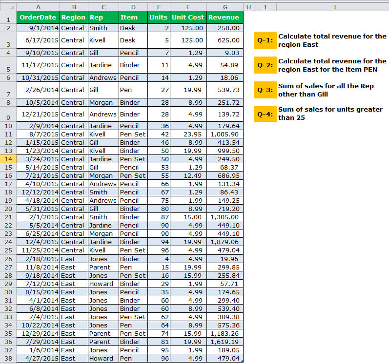
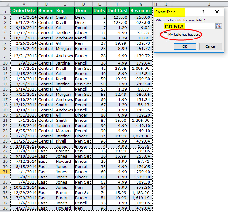
Set up the Data: Since we already have our criteria, we need first to set up the data table. We must select the data and make it in a table format. Then, click the "Ctrl + T" and choose the data.
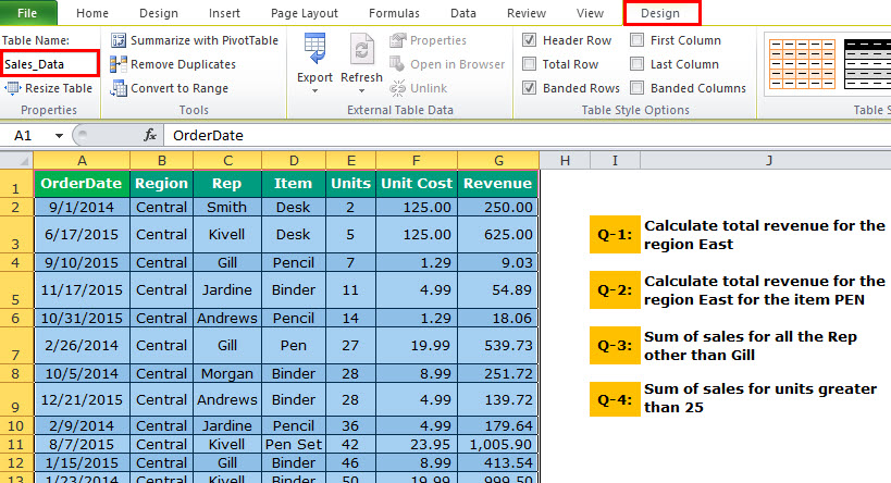
And, name the table "Sales_Data."
Create Your Criteria: After setting up the table, we need to create our criteria. Our first criteria will be like the one below.
Q1 – Our first question is to calculate the revenue for the region "Central."
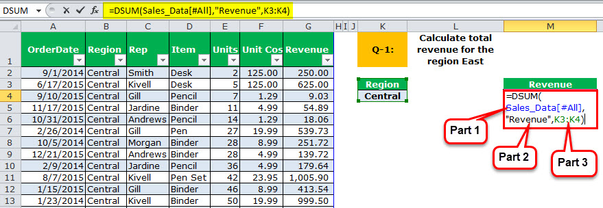
We must apply the DSUM formula to get the region "Central" total.
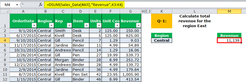
The output is 11,139.
Part 3: To sum up, we must specify the criteria as the "Central" region.
Part 2: It specifies which column you need to sum, i.e., the "Revenue" column in the table.
Part 1: It is taking the range of databases. We name our database "Sales_Data."
Note: All the characters should be the same as in the data table for the "criteria" column.
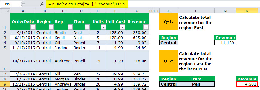
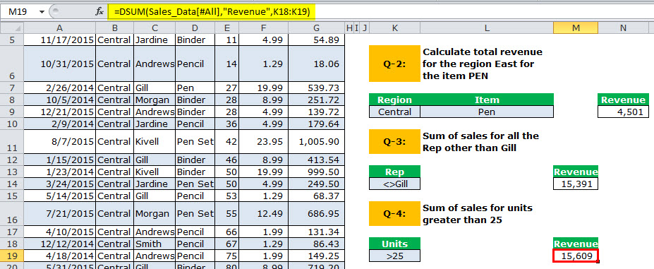
Q-2: Calculate total revenue for the region "East" for the item "Pen."
We need to calculate the total revenue for the region "East" but only for "Pen" in the item column.
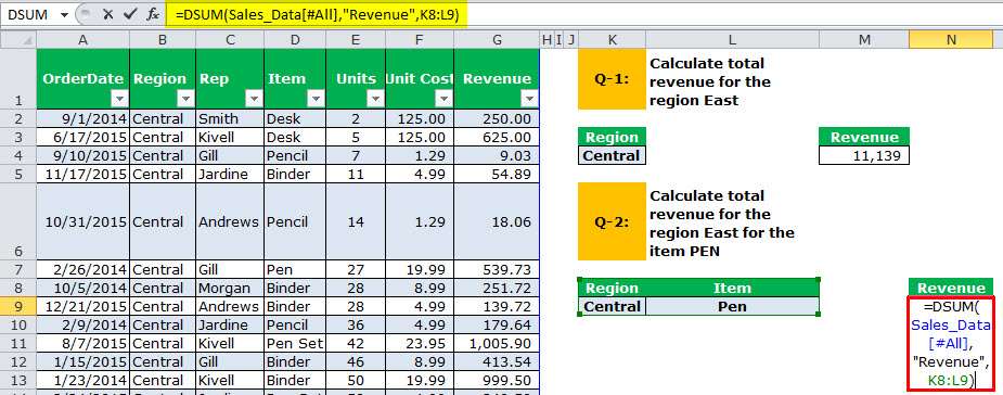
The output is 4,501.
Q-3: Sum of sales for all the Rep other than Gill.
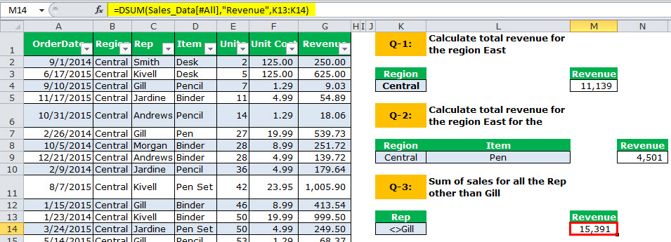
We need to calculate the "Sum for all the Rep other than Gill." We need to give criteria under "Rep" as <>Gill.
“<>” means not equal to.
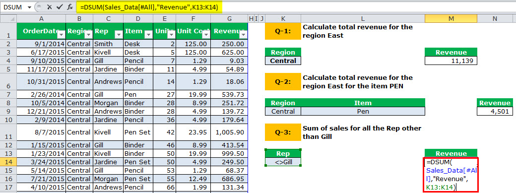
The output is 15,391.
Q-4: Sum of sales for units greater than 25.
The equation calculates the total revenue for all the units greater than 25 units.
For this, set the criteria as >25.
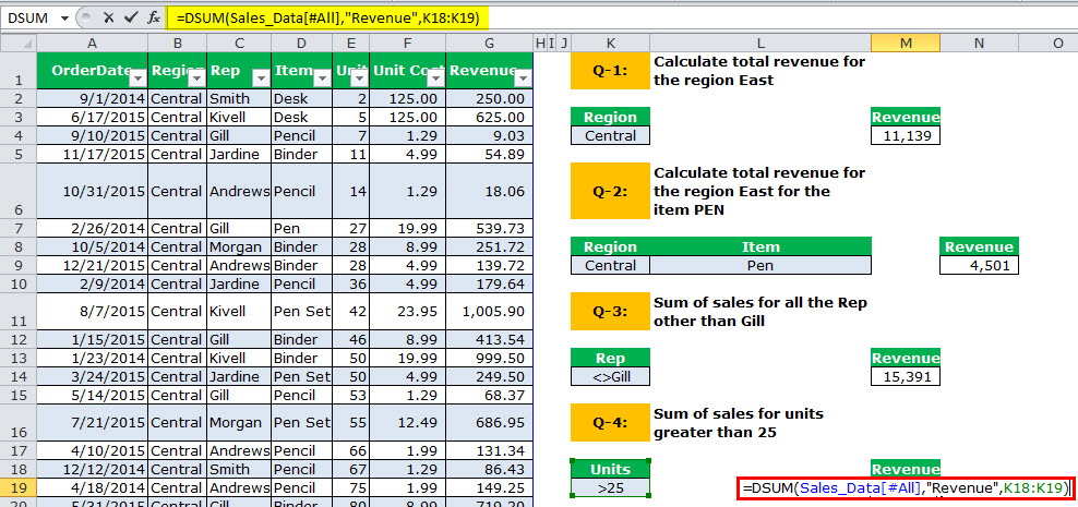
The output is 15,609.
Q-5: Sum of sales from 18th Oct 2014 to 17th Oct 2015
We need to get the total revenue from 18th Oct 2014 to 17th Oct 2015. To do this, we need to set two criteria for one column.
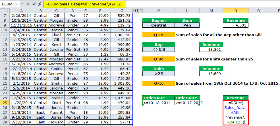
The output is 8646.

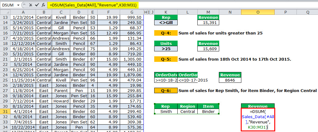
Q-6: Sum of sales for Rep Smith, for item Binder, for Region Central
Now, we have to match 3 different criteria to get the total.

We must design the criteria as shown in the below table and apply the DSUM function.

Things to Remember
- While writing a field name, it must be in double quotes and should be as same as in the table header.
- First, identify the criteria requirement and list all the criteria.
- We must create a table for the data. If the data size increases, it will be a dynamic range. You need not worry about the range.
- The #Value error occurs due to wrong field names included in the database argument.
- If we do not give any specific criteria, it will just give us the overall sum for the column.
- We must create a drop-down list of your criteria to get different regions or different rep totals.
- As soon as we change the drop-down list, it may show the results accordingly.
- The criteria table is not case-sensitive.
- It is an alternative formula for SUMIF and SUMIFS functions.

