Discrete Distribution

Discrete Distribution Definition

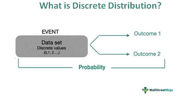
Discrete distribution in statistics is a probability distribution that calculates the likelihood of a particular discrete, finite outcome. In simple words, the discrete probability distribution helps find the chances of the occurrence of a certain event expressed in terms of positive, non-decimal, or whole numbers as opposed to a continuous distribution.

Discrete distribution is a very important statistical tool with diverse applications in economics, finance, and science. For example, it helps find the probability of an outcome and make predictions related to the stock market and the economy. Major types of discrete distribution are binomial, multinomial, Poisson, and Bernoulli distribution.

• Discrete distribution depicts the occurrence of a certain event that one can express as distinct, finite variables.
• The accepted discrete values are restricted to whole numbers. Hence, negative values, fractions, or decimals are not considered.
• Probability distributions are of two types – discrete and continuous. The latter differs from the former in that it calculates the probability of any value (negative, decimal, etc.).
• The distribution is used in many experiments in the field of science and by finance experts to analyze certain discrete metrics and also to evaluate the stock market.

Discrete Distribution Explained

The discrete distribution function is one of the many mathematical tools adopted in finance and economics. For example, an idea of the discrete probability can help in forecasting, as used by stock market experts and experienced investors. Let us try to understand the basics of discrete distribution.

If a person is given a set of data consisting of only whole numbers and asked to find the probability of something, it becomes a discrete probability. For example, when a person throws a die, it can show any value from 1 to 6. The numbers 1, 2, 3, 4, 5, and 6 are discrete whole numbers.

On the contrary, if the same person is given another data set containing the exact temperatures of a city over a week, it can be any value. This is because temperatures are not always whole numbers like 320 or 800. The data set given to the person comprises temperatures in the following manner:

81.2⁰, 83.4⁰, 85⁰, 88.9⁰, 91.6⁰, 89.3⁰, 82⁰

The discrete probability distribution does not apply to this data set, as they are decimals.

Discrete distribution of throwing a die

Now, let’s see how to calculate discrete distribution using the example of throwing a die.

The sample space here is S = {1,2,3,4,5,6}

In other words, it is the list of all possible outcomes.

Number on the die	1	2	3	4	5	6
Probability	1/6	1/6	1/6	1/6	1/6	1/6

Adding the individual probabilities, we get 6/6 = 1.

A few important points to remember:

• The probability of an outcome can be a decimal value. But the input values should be whole numbers. So, for example, while throwing a die, the input values (1 to 6) are positive, non-decimal numbers, but the probability of getting any number (say, 6) when a die is rolled is 1/6 or .133.
• The probability of a particular outcome should always lie between 0 and 1 (both inclusive). So, for example, the probability of getting a six when a die is thrown is 0.133.
• The sum of the individual probabilities should equal 1. So, again, considering the example of throwing a die, we get the sum as (6 x 1/6) = 1.

Types

Here are the types of discrete distribution discussed briefly. There are four main types:

#1 - Binomial distribution:

The binomial distribution is a discrete probability distribution that considers the probability of only two independent or mutually exclusive outcomes - success and failure. The value given to success is 1, and failure is 0.

P(x) = ⁿC_{x ·} p^x (1 − p)^n−x

Where n= number of events

P=probability

X= number of successful event.

#2 - Multinomial distribution

The multinomial distribution is similar to the binomial distribution, except that it calculates the likelihood of occurrence of more than two outcomes.

p= n! (p1x1 × p2x2 × …pk x k) / (x1!× x2! …× x k!)

Where x1: number of times outcome 1 happens

p1: probability of outcome 1 occurring

#3 - Bernoulli distribution

Bernoulli distribution is similar to the binomial discrete distribution in that it considers only two variables. Therefore, it has two outcomes – success and failure. However, in the Bernoulli distribution, only a single trial is conducted to find the probability of an outcome, as opposed to the binomial distribution in which multiple trials are conducted.

F(k,p)= pk + (1-p) (1-k)

Where p=probability

K= possible outcomes

F= function

#4 - Poisson distribution

Poisson distribution shows the probability of the number of times an event is likely to occur in a specified time interval.

P(x; μ) = (e-μ * μx) / x!

Where μ = expected number of events

Examples

Let’s discuss some examples :

Example #1

Consider the expected number of people who visit the gym at different times of the day.

Time	6:00 a.m.	7:00 a.m.	8:00 a.m.	9:00 a.m.	4:00 p.m.	5:00 p.m.	6:00 p.m.	7:00 p.m.	8:00 p.m.
No. of people	25	30	10	5	5	15	30	25	5

Here, the number of people who visit the gym at any time cannot be expressed as a decimal, and it can’t be negative either. Hence, the distribution is discrete.

Example #2

Discrete probability distribution, especially binomial discrete distribution, has helped predict the risk during times of financial crisis. Also, it helps evaluate the performance of Value-at-Risk (VaR) models, like in the study conducted by Bloomberg. It estimates the performance of different VaR models during many financial and non-financial crises that occurred from 1929 to 2020.

Continuous vs Discrete Distribution

There are two types of probability distribution applicable for any given data: discrete and continuous. Let’s differentiate between these two types of distribution:

Discrete distribution	Continuous distribution
The likely outcomes of an event must be discrete, integral values.	The likely outcomes of an event can be any mathematical value.
Acceptable values are whole numbers (positive, non-decimal).	Negative and decimal values are accepted.
Applicable for a finite data set.	Applicable for infinite data set.

Suppose an investor considers the historical value of Amazon’s stock from the first day it was traded. The investor collects a vast amount of data on the different prices in a day. The data set would contain many decimal numbers. Similarly, if a scientist calculates the weight of microscopic particles, they would get values in the range of 10^-6. So here, too, continuous distribution can be used. These are examples of continuous distribution.

Frequently Asked Questions (FAQs)

Recommended Articles

This has been a guide to discrete distribution and its definition. We explain how to calculate it, its types, examples, and vs. continuous distribution. You may learn more from the following articles -

• Uniform Distribution
• Sampling Distribution
• Probability Distribution