Dickey-Fuller Test

Published on :

21 Aug, 2024

Blog Author :

Edited by :

Reviewed by :

The Dickey-Fuller (DF) Test refers to a statistical test used to ascertain the stationarity in an autoregressive time series model. In other words, it examines the data series for the rejection of the null hypothesis and the existence of unit root when the outcome is more negative compared to the critical value.

As the result of such statistical testing is more negative when compared to the critical value, the null hypothesis is rejected, proving the stationarity or trend-stationarity of the given time series. Also, the alternative hypothesis in this unit root testing method can vary according to the applied equation. It is a widely used metric in finance and econometrics.

Dickey-Fuller Test Meaning

The Dickey-Fuller (DF) test refers to a unit root test that facilitates the identification of stationarity in a given time series data.
If the resulting test statistic is not as negative as the critical value, the null hypothesis is rejected, interpreting the unit root presence in the data. However, the null hypothesis is rejected if the test statistic is considerably more negative than the critical value, confirming the series' stationarity.
Conversely, the Augmented Dickey-Fuller (ADF) test is the extended and improved form of the DF test, which provides a more reliable outcome when the data is of high order, complex, or extensive.

Dickey-Fuller Test In Finance Explained

The Dickey-Fuller Test for stationarity is frequently employed in finance to ensure that the critical statistical properties, such as mean and variance, in time series data remain constant over time. This assumption is inevitable for accurate financial modeling and forecasting.

It enables the comprehensive examination of past trends in finance and confirms whether these trends remain relevant as markets move forward. Also, if data lacks stationarity, the testing undertaken as part of financial modeling and forecasting may give unreliable results.

By determining stationarity, the Dickey-Fuller test assists analysts in determining whether data transformation, such as differencing, is necessary to prepare the data for further analysis or modeling. When dealing with stationary data, trading signals are formulated on the assumption that stock prices will eventually revert to the mean. This allows for capitalizing on price deviations from the mean within short time frames.

The Dickey-Fuller test was developed by American statisticians David Dickey and Wayne Fuller in 1979. Since then, it has served as a fundamental method for detecting whether the data has a unit root, which is crucial for assessing its stationarity.

It has been widely used for trending time series like asset prices. However, many economic and financial time series are more complex than the simple autoregressive models. Therefore, the duo extended this model to eliminate the various limitations and came up with the Augmented Dickey-Fuller (ADF) Test, which provides a more comprehensive analysis for extensive and high-order data. It must be noted that both DF and ADF work well when data is linear, indicating that data nonlinearity may skew the results.

Formula

Unit root testing in statistics is essential for analyzing the stationarity of data, which is a prerequisite for various statistical testing measures. The Dickey-Fuller test calculation involves the use of the following equation:

ΔY_t = α + pY_t-1 + Ɛ_t ; H₀: p = 1 → implies that the data is non-stationary

H₁: p ≠ 1 → depicts that the data is stationary

Where,

Yt is the given data;
α is the drift or intercept constant;
p is the coefficient signifying the unit root;
Y_t-1 is the value at lag of 1 in the time series;
Ɛ_t is the error term or noise

The Dickey-Fuller test interpretation involves the rejection of the null hypothesis to prove the stationarity of data.

Examples

Moving ahead, let us understand the Dickey-Fuller test for stationarity through some examples.

Example #1

Let us consider the following graph depicting the month-on-month performance of Starlight Corp’s stock.

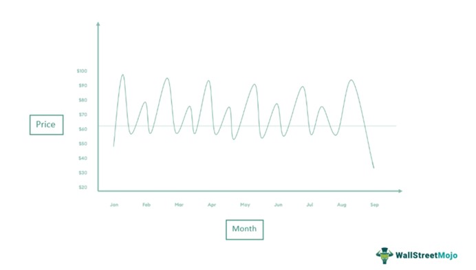
Dickey-Fuller test Interpretation: One can visually identify that the time series is stationary. Thus, on conducting the DF test, they have a coefficient of less than 1, signifying the rejection of the null hypothesis, i.e., the data has the presence of a unit root.

Example #2

Suppose Jenny, a market researcher, wants to interpret the next month's potential performance of the stock of WinFin Ltd. using the Autoregressive Integrated Moving Average (ARIMA) model.

She acquires the sample data for the last 3 months and uses it to evaluate future stock prices. However, to ensure that the time series data is stationary, Jenny performs the DF test and records the results. Thus, the unit root test enabled her to ensure that the data was predictable and relevant in the future.

Dickey-Fuller Test vs Augmented Dickey-Fuller Test

The Dickey-Fuller test and the Augmented Dickey-Fuller test serve similar purposes in determining whether a time series dataset exhibits a unit root, indicating non-stationarity. However, there are several key differences between the two. They have been listed in the table below.

Basis	Dickey-Fuller Test	Augmented Dickey-Fuller Test
Definition	The Dickey-Fuller test is a unit root testing process for gauging the stationarity in a time series data.	The Augmented Dickey-Fuller (ADF) test is an extended and improvised version of the DF test that facilitates the unit root testing of high-order complex regressive models by considering additional lagged terms of the differential series, ensuring autocorrelation.
Determines	It determines stationarity in time series data.	Both stationarity and non-stationarity of the data can be determined.
Model	It employs a simple autoregressive model.	It uses a high-order regressive process in the time series model.
Efficiency	The DF test is less efficient compared to the ADF test for interpreting stationarity in large or complex data series.	It is a more efficient test that gauges data stationarity for high-order, large, or complex autoregressive time series models.
Null Hypothesis	The null hypothesis is rejected when the coefficient is not equal to 1, depicting stationarity in data.	The null hypothesis is rejected when the test statistics are less compared to the critical value, signifying the presence of stationarity in the time series.
Critical Values	It derives critical values from the standard Dickey-Fuller test table.	The ADF test evaluates the critical values, which are taken from the Dickey-Fuller test table and adjusted according to the augmented model.
Formula	ΔY_t = α + pY_t-1 + Ɛ_t	Y_t= c + β_t+ αY_t−1+ pΔY_t−1+ e_t
Usability	It is a less commonly used method compared to the ADF test.	As it is highly flexible and reliable, the ADF test is widely used in finance and econometrics, like for stock pairing in trading.

Frequently Asked Questions (FAQs)

What is the rejection rule for the Dickey-Fuller (DF) test?

The DF test assumes that the data has unit root presence (H0: p = 1); however, this null hypothesis is rejected in case the test statistic (p-value) is less than the significance level.

What is the critical value in the Dickey-Fuller test?

The Dickey-Fuller critical values are as follows:

a. -3.43 at the 0.01 level;
b. -2.86 at the 0.05 level;
c. -2.57 at the 0.10 level.

These values depend on the sample size and significance level.

What are the limitations of the Dickey-Fuller (DF) test statistic?

The primary pitfall of a DF test for stationarity is that it lacks statistical power for interpreting the unit root efficiently when the autoregressive time series data is of high order or the sample is too large. There are some other limitations as well, such as the normality of error assumption.

Why use the Dickey-Fuller test?

The DF test is critical for determining the stationarity in a given time series like the Autoregressive Integrated Moving Average (ARIMA) model. In the absence of stationary data, i.e., if the sample data is non-stationary, such data cannot be used for predicting future asset prices in stock analysis. In finance, stationarity facilitates risk management, investment strategizing, and market analysis, among other things.