Date Format in Excel

What is the Date Format in Excel?

In Excel, a date is displayed according to the format selected by the user. One can choose from the different formats available or create a customized format according to the requirement. The default date format is specified in the “Control Panel” of the system. However, it is possible to change these default settings.

For example, the date 01/01/2021 corresponds to the format dd/mm/yyyy. If the format is changed to d-mmm-yyyy, the date becomes 1-Jan-2021.

We can change the date format in Excel either from the “Number Format” of the “Home” tab or the “Format Cells” option of the context menu.

In Excel for Windows, 1900 is the default date system. Whereas, in Excel for Mac, 1904 is the default date system. Both these systems store the dates as consecutive numbers having a difference of 1. These numbers are known as serial values or serial numbers. The reason dates are stored as serial numbers is to facilitate calculations.

In the 1900 date system, the first date that Excel recognizes is January 1, 1900. This date is stored as the number 1 in Excel. Consequently, the number 2 represents January 2, 1900. The last date recognized by Excel is December 31, 9999. It is represented by the serial number 2958465. Date before 1900 or after 9999 is identified as a text value by Excel.

Dates are stored only as positive integers in the 1900 date system. However, to display negative numbers as negative dates, one needs to switch to the 1904 date system.

In the 1904 date system, 0 represents January 1, 1904, and -1 means January -2, 1904. The number 1 represents January 2, 1904. The last date recognized by Excel (in the 1904 date system) is December 31, 9999, represented by the serial number 2957003.

In this article, we follow the 1900 date system.

What is theDate Format in Excel?

Code of Date Format in Excel

A code (like dd-mm-yyyy) is a representation of a day (d), month (m), and year (y). We can change the appearance of the date by changing the specified code.

The different codes, their explanation, and output (for days, months, and years) have been presented in the following images.

Notations for a Day

Notations for a Month

Notations for a Year

How to Change Date Format in Excel?

Here we look at some of the date format examples in Excel and how to change them.

Example #1–Apply Default Format of Long Date in Excel

The following image shows a number in cell A1. We want to know the date represented by this number. The output should be in the long date format of Excel.

The steps to know the date represented by the number in cell A1 are listed as follows:

We must first select cell A1. Then, from the “Home” tab, click the “Number Format” drop-down appearing in the “Number” section. Next, select “Long Date,” shown in the following image.
The output is shown in the following image. The long date format displayed is dd mmmm yyyy. Hence, the number 1 represents the date 01 January 1900 in the long date format.
Note: The short and long dates appear as set in the “Control Panel.” Click “Clock, Language, and Region” in the “Control Panel” to change these default date formats. After that, click “Change date, time, or number formats.” Make the desired changes and click “OK.”

Likewise, had there been 2 in cell A1, the long date format would have been 02 January 1900. The number 3 would have been displayed as 03 January 1900 in the long date format.

Note: To switch to the 1904 date system, we must select “Advanced” from the “Options” of the “File” tab. Under “When calculating this workbook,” select “use 1904 date system” and click “OK.”

You can download this Change Date Format Excel Template here – Change Date Format Excel Template

Example #2–Change the Date Excel Format Using “Custom” Option

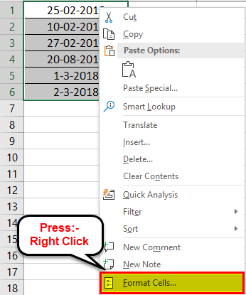
The following image shows some dates in the range A1:A6. These dates are in the format dd-mm-yyyy. We want to change their format to dd-mmmm-yyyy.

For instance, the date in cell A1 should appear as 25-February-2018. We may use the “Custom” option of the “Format Cells” dialog box.

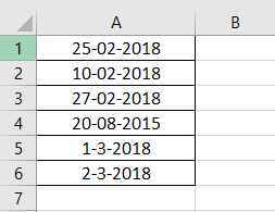
The steps to change the date format in Excel are listed as follows:

Step 1: We need to select all the dates of the range A1:A6. The same is shown in the following image.

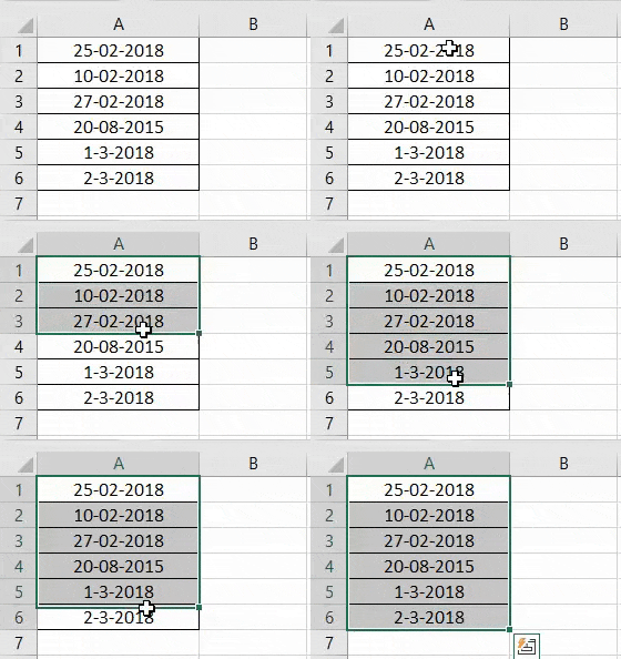
Step 2: We must right-click the selection and choose “Format Cells” from the context menu. Alternatively, we may also press the keys “Ctrl+1” together.

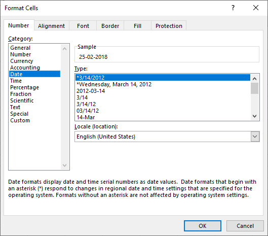
Step 3: The “Format Cells” window opens, as shown in the following image.

Note: The default short date and long date formats are marked with an asterisk (*) in the box under “type.” The short date is 3/14/2012 (m/dd/yyyy), and the long date is Wednesday, March 14, 2012 (dddd, mmmm dd, yyyy).

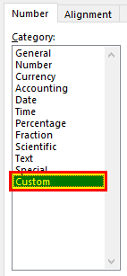
Step 4: From the “Number” tab, we need to select “Custom” under “Category.” The categories are shown on the left side of the “Format Cells” window.

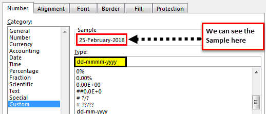
Step 5: Under “Type,” we must insert the required date format. Either type the format (dd-mmmm-yyyy) or select it from the various options displayed in the box below “Type.”

Once the format has been entered, check the preview of the first date (of the range A1:A6) under “Sample.” The same is shown in the following image. Click “OK” in the “Format Cells” window if the date preview looks good.

Note 1: The date under “Sample” is displayed according to the format specified under “Type.”

Note 2: While creating custom date formats, we can use a forward slash (/), hyphen (-), comma (,), space ( ), etc.

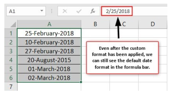
Step 6: The output is shown in the following image. All dates of the range A1:A6 have been converted to the format dd-mmmm-yyyy. However, the Excel formula bar can still see the default date format. This default format corresponds with the short date set in the “Control Panel.”

Example #3–Apply Different Types of Customized Date Formats in Excel

The next image shows certain dates in the range A1:A6. At present, the date format is dd-mm-yyyy.

We want to apply four different formats to these dates. For using each format, the common steps to be performed are given as follows:

First, we must select the range A1:A6.
Then, right-click the selection and choose “Format Cells.”
After that, from the “Number” tab, select “Custom” under “Category.”

Further, under each format, the additional steps to be performed followed by two images are given.

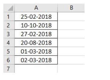
Format 1: dd-mmm-yyyy

In the “Custom” option of the “Number” tab, select the format “dd-mmm-yyyy” under “Type.”
Click “Ok.”

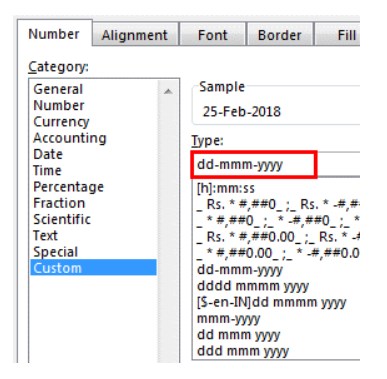
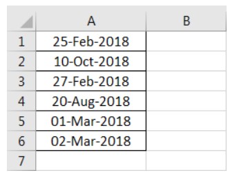
The output is given in the following image. All dates are displayed according to the format dd-mmm-yyyy. The hyphen is the separator between the day, month, and year in this format.

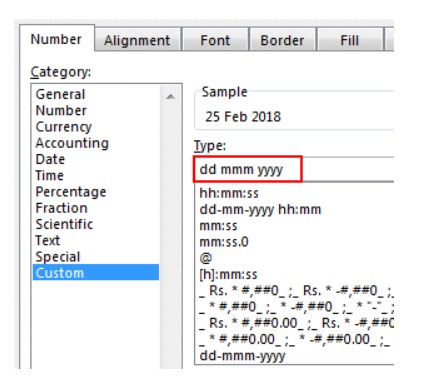
Format 2: dd mmm yyyy

We must select the format “dd mmm yyyy” under “Type” of the “custom” option.
Click “Ok.”

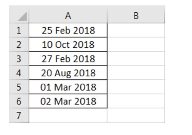
The output is given in the following image. All dates are converted to the format dd mmm yyyy. The space is the only separator between the day, month, and year in this format.

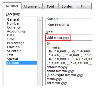
Format 3: ddd mmm yyyy

In the “Custom” option, select the format “ddd mmm yyyy” under “Type.”
Click “Ok.”

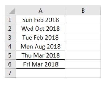
The output is given in the following image. The dates are shown in the format ddd mmm yyyy. The day and the month are displayed in their short notations in this format.

Format 4: dddd mmmm yyyy

From the “Custom” option of the “Number” tab, select “dddd mmmm yyyy” under “Type.”
Click “Ok.”

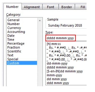
The output is given in the following image. All dates have been converted to the format dddd mmmm yyyy. The date, month, and year are displayed in their respective full forms in this format.

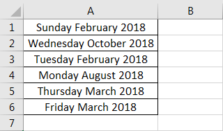
It must be observed that the date format changes as per the style set by the user. Therefore, the user can select a date format according to their convenience.

Example #4–Convert Text Values Representing Dates to Actual Dates

The following image shows a list of dates in the range A1:A6. At present, these dates are appearing as text values. We want to convert these text values to dates having the format dd-mmm-yyyy.

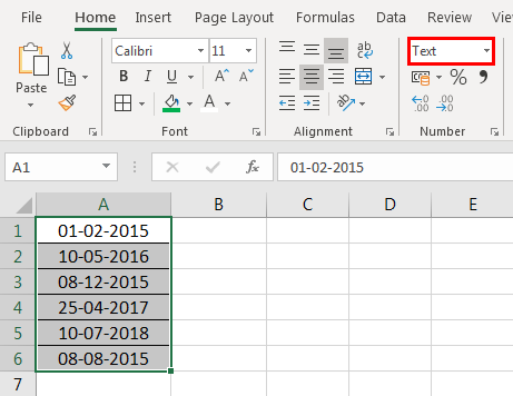
The steps to convert text values to dates having the given format are listed as follows:

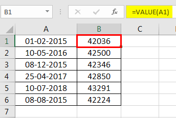
Step 1: First, enter the following formula in cell B1.

“=VALUE(A1)”

Then, press the “Enter” key.

Note 1: The VALUE functionVALUE Excel Function In Excel, the value function returns the value of a text representing a number. So, if we have a text with the value $5, we can use the value formula to get 5 as a result, so this function gives us the numerical value represented by a text.read more returns the numeric form of a text string that represents a number. In other words, it converts a number looking like the text into an actual number.

Note 2: Instead of the VALUE function, one can also use the DATEVALUE functionDATEVALUE Excel The DATEVALUE function in Excel shows any given date in absolute format. This function takes an argument in the form of date text normally not represented by Excel as a date and converts it into a format that Excel can recognize as a date.read more of Excel. The latter converts a date stored as text to a serial number. This serial number is recognized as a date by Excel.

Step 2: We must select cell B1 and drag the fill handle until cell B6. The output is shown in the following image. All text values (A1:A6) have been converted to numbers (in the range B1:B6).

Ideally, the text string in Excel is left-aligned while the number string is right-aligned. However, we have centrally aligned both the ranges (A1:A6 and B1:B6).

Note: When text strings representing dates have been converted to serial values (or dates), we can use them for performing different calculations like addition, subtraction, and so on.

Step 3: To view the obtained serial numbers (in column B) as dates, apply the required format. We must select the range B1:B6, right-click and choose “Format Cells.”

In the “Number” tab, select the option “Custom.” Then, under “Type,” enter or choose the format “dd-mmm-yyyy.” The same is shown in the following image.

If the sample date looks alright, click “OK.”

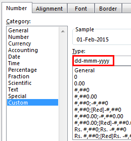
Step 4: The output is shown in the following image. Hence, all text values (of column A) have been converted to valid dates (in column B) having the format dd-mmm-yyyy.

Note: To ensure that a value is recognized as a date by Excel, check for the following signs:

The dates are right-aligned as they are numerical values.
If two or more dates are selected, the status bar (at the bottom of the worksheet) shows the count, average, numerical count, and sum. In addition, it may display one or more options according to the Excel version.

If a value is a text string, it would be left-aligned, and the status bar will show only the count.

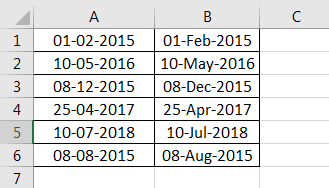
Often, the Excel date format needs to be changed (from text to dates) when data is downloaded (or copied and pasted) from the web. That is because, in such instances, the dates may not be displayed as numbers.

Example #5–Change the Date Format Using “Find and Replace” Box

The following image shows some text values representing dates in the range A1:A6. The days, months, and numbers have been separated with a backslash. That is because we want to perform the following tasks:

Replace all the backslashes () with forwarding slashes (/) by using the “Find and Replace” dialog box.
Convert text values representing dates to actual dates.

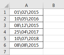
The steps to perform the given tasks are listed as follows:

Step 1: We must press the keys “Ctrl+H” together. Then, the “fin d and replace” dialog box opens, as shown in the following image.

Step 2: Type a backslash in the “Find what” box (). In the “Replace with” box, type a forward slash (/).

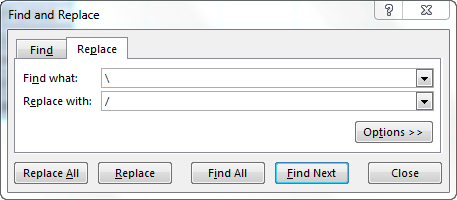
Step 3: Next, we must click “Replace All.” Excel shows a message stating the number of replacements it has made. Click “OK” to proceed. The final output is shown in the following image.

Hence, all backslashes have been replaced with forwarding slashes. With this replacement, the text values representing dates have automatically been converted to actual dates by Excel.

Since column A was aligned centrally from the beginning, this alignment is retained even after the values are converted to dates.

Frequently Asked Questions

1. How can the date format in Excel be changed?

The steps to change the date format in Excel are listed as follows:
The steps to change the date format in Excel are listed as follows:

a. Select the cell containing the date. If the date format of a range needs to be changed, select the entire range.
b. Right-click the selection and choose “Format Cells” from the context menu. Alternatively, press the keys “Ctrl+1” together.
c. IIn the “Number” tab, select the option “Date.” Next, select the required date format under “Type.”
d. Check the preview (of the first date of the selected range) under “Sample.” If the preview is good, click “OK.”

The date format of the selected cell or cells (selected in step a) is changed.

Note 1: The required date format may not be available under the “Date” option’s “Type.” If it is not available, select “Custom” as the “category” from the “Number” tab. Then, type the required date format under “Type” and click “OK.”

Note 2: If the selected cell (selected in step a) contains a text string representing a date, convert this string to date first. Then change the format to the desired date format.

2. How to change the date format permanently in Excel?

To change a date format permanently, one needs to make changes to the date formats of the “Control Panel.” That is because the short and long date formats of Excel reflect the date settings of the “Control Panel.”

The steps to change the date settings of the “Control Panel” are listed as follows:

We must open the “Control Panel” first from the “Start” menu.
b. In the “Clock, Language, and Region” category, click “Change date, time, or number format.” It is available under the “Region and Language” option.
c. The “Region and Language” or “Region” dialog box opens. Under “Format,” we must select the region.
d. Enter the required short and long date formats under “Date and Time Formats.” To enter customized short and long date formats, click “Additional Settings.” The “Customize Format” dialog box opens. Make the changes in the “Date” tab and click “OK.”
e. Check the preview under “Examples” at the bottom of the “Region and Language” box. If the preview is alright, click “OK.”

The default date settings have been changed. Now, we should enter a date in any format in Excel. Then select the short or the long date format from the “Number Format” (in the “Number” section) of the “Home” tab.
The dates will appear in the format set in the “Control Panel.” So, the user need not change the format of each date manually.

3. How to change a date to a text string in Excel?

Let us change the date 22/1/2019 in cell A1 to a text string in Excel. The text string should be in the format yyyy-mm-dd.

The steps to change a date to a text string are listed as follows:
a. First, we must enter the formula =TEXT(A1, “yyyy-mm-dd”) in cell B1.
b. Then, press the “Enter” key.

The date in cell A1 (22/1/2019) is converted to 2019-01-22 in cell B1. We must note that the date in cell A1 is right-aligned, being a number. In contrast, the text in cell B1 is left-aligned.

Note: The TEXT function helps convert numbers to text strings. It is used to display values in a specific format. The syntax is TEXT(value,format_text). “Value” is the number to be converted to text. “Format_text” is the format in which the number should be displayed.

Date Format in Excel