Table Of Contents
What Is Custom Number Format In Excel?
Custom Number Format in Excel is a feature where we format the selected data values to customized numeric formats because the output of the executed formula, or the entered value in a cell, gets entered as per the default formatting of the cell.
The Excel Custom Number Format is useful as it helps users to get the right formatting of the cell value, or also to pre-set the customized numeric format before entering the desired values.
Key Takeaways
- We can Custom Number Format in Excel by creating or customizing the existing number formats in Excel as the output cells or empty cells where we enter the values may have the default formatting of the cell.
- When we customize the numeric format, we can highlight the results using the Format Painter or Conditional Formatting Options available in Excel.
- We can customize format for Dates, Time, and Numeric Figures in Millions, Billions, etc.
- We can also display only the numeric values, hide the textual values, and differentiate positive and negative values with Plus Sign and brackets, respectively.
How To Custom Format Numbers In Excel?
To make the data presentable or visually appealing, we can get Custom Number Format in the following ways, namely:
- Using the inbuilt Number Format in Excel, or
- Creating new numeric formats by customizing as desired.
Excel works on numbers and is based on the format we give. It shows the result.
For example, look at the below example.
In cell C1, we have the number 43473.

As of now, the Excel format of the custom number is “General”.

If we click on the drop-down list, there are several built-in number formats available here, like “Number,” “Currency,” “Accounting,” “Date,” “Short Date,” “Time,” “Percentage”, etc.
These are all predefined formatting, but we can customize all these and make the alternative number formatting, which is called “Custom Number Formatting.”
How To Create A Custom Number Format In Excel? (Using Shortcut Key)
Normal formatting is available under the “Home” tab. We must right-click on the specific cell and select “Format Cells” for custom formatting.
The shortcut key to formatting, i.e., to open the Format Cells window, is Ctrl + 1.

Examples
We will Custom Number Format in Excel for various cell values with specific examples.
Example #1 - Date Custom Format
It is the most common formatting we work with day in and day out.
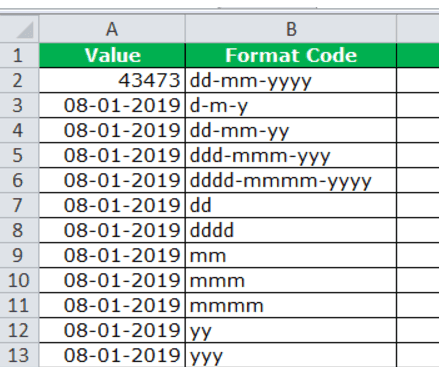
Now, look at the below image. We have a number in cell C1.

We want to display this number as a date. So, select the cell, and press Ctrl + 1.

Next, select the “Custom” format in Excel, and type the required date format in the “Type:” field.

- DD means the date should be first and two digits.
- MM means the month should be second and two digits.
- YYYY means the year should be last and four digits.
Now, press the “Enter” key. It will show the date in the selected format, as shown below.

Example #2 - Time Custom Format
We can customize the format of the time as well. Below are the available codes for the time format.

If you observe the above table, we have not mentioned the code to show the minute. Unfortunately, we cannot show only the minute section since “m” & “mm” coincide with the month.
In scenarios where the time exceeds 24 hours, we mention the hours in brackets, i.e., .
Example #3 - Number Custom Format
When we work with numbers, it is very important to show the numbers to the readers. There are several ways we can show up the numbers. The codes below will help you design your number format.

Example #4 - Show Thousand Numbers in K, M, and B Format
Showing numbers in lakhs can sometimes require a lot of cell space and not fit in the report, but we can customize the number format, using the codes shown in the below image, to make it fit.

Example #5 - Show Negative Numbers in Brackets & Positive Numbers with + Sign
We can display the negative numbers in brackets and positive numbers with the + sign to make them clearly comprehendible using the codes shown in the image below.

#6 - Show Numbers Hide Text Values
Sometimes, showing only numerical values and hiding all the text values technique is required. So, the below code can help us with this.

#7 - Show Numbers with Conditional Colors
We have seen cases where we wanted to show some values in “blue” and some in “green.” By changing the number format, we can alter the font colors.

Important Things To Note
- Displaying huge numbers with numeric names like Millions and Billions will make the report more appealing instead of keeping track of the zeros and read them.
- We can display different numbers in different colors too.

