Table Of Contents
What is COUNTIF Function in Excel
The COUNTIF function in Excel counts the number of cells within a range based on pre-defined criteria. It is used to count cells that include dates, numbers, or text. For example, COUNTIF(A1:A10,"Trump") will count the number of cells within the range A1:A10 that contain the text "Trump"
Syntax
The syntax of COUNTIF formula in Excel is stated as follows:

It accepts the following required arguments:
- Range: It represents the range of values on which the criteria will be applied.
- Criteria: It represents the condition that is applied to the range of values. The values that meet the criteria are returned as a result.
The output of the COUNTIF formula is a positive number which can be zero or non-zero.
How to Use COUNTIF Function in Excel?
Being a worksheet (WS) function, the COUNTIF function can be entered as a part of the cell formula. The usage of the COUNTIF function is the same in Excel and VBA (COUNTIF function VBA).
Let us consider some uses to understand the working of the COUNTIF excel function.
#1 - Count Values with the Given Value
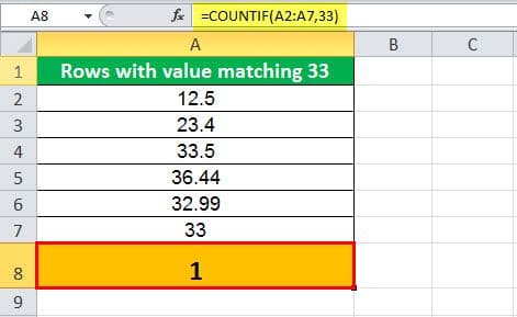
The following table shows a list containing numerical values in the cells A2:A7. Count the given range of cells for the values matching the number “33”.
The COUNTIF function is applied to the given range of cells, and the formula is stated as follows:
“=COUNTIF (A2:A7,33)”
Here the condition applied to the formula is the number “33”.The formula checks the range of cells A2:A7 for the values matching number “33”. The range contains only one such number, which satisfies the condition. Hence the result returned by the COUNTIF function is “1”. The result is displayed in cell A8.

#2 - Count Numbers with a Value Less Than the Given Number
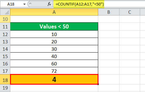
A list of data in the cells A12:A17 is provided in the succeeding table. Count the given range of cells for the values less than “50”.
The COUNTIF function is applied to the given range of cells, and the formula is stated as follows:
“=COUNTIF(A12:A17,“<50”)”
Here the condition applied to the formula is “<50”. The COUNTIF formula checks the range of cells matching the condition, less than 50. There are only four values that are less than 50 in the range. Hence the result returned by this function is “4”. The result is displayed in cell A18.
#3 - Count Values with the Given Text Value
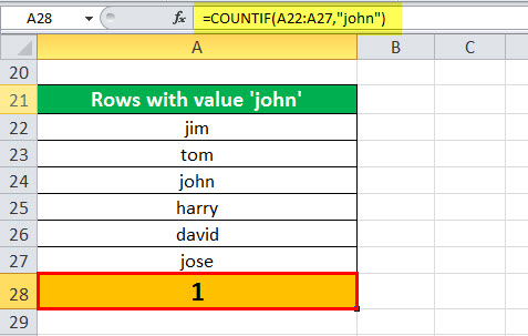
A list of data in the cells A22:A27 is provided in the below table. Count the range of cells for the text value “john”.
The COUNTIF function is applied to the given range of cells, and the formula is stated as follows:
“=COUNTIF(A22:A27, “john”)”
Here the condition applied to the formula is the value “john.” The COUNTIF formula checks the range of cells matching the given condition. The given range has only one cell that satisfies the text value “john”. Hence, the result is “1” which is displayed in cell A28.
#4 - Count Negative Numbers
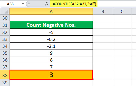
A list of data in the range of cells A32:A37 is provided in the below table. Count the range of cells for negative values (that is, less than zero).
The COUNTIF function is applied to the given range of cells, and the formula is stated as follows:
“=COUNTIF(A32:A37, “<0”)”
Here the condition applied to the formula is less than zero. Now, the COUNTIF formula will identify and count the numbers with negative values in the given range. There are three such numbers in the given range. Hence, the result is “3” which is displayed in cell A38.
#5 - Count Zero Values
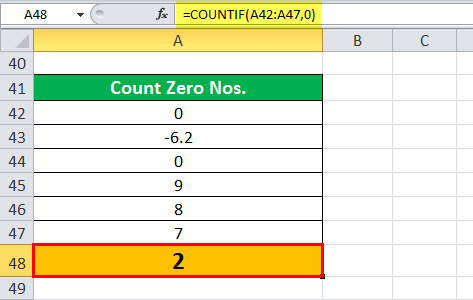
A list of data in the range of cells A42:A47 is provided in the below table. Count the range of cells for the value “0”.
The COUNTIF function is applied to the given range of cells, and the formula is stated as follows:
“=COUNTIF(A42:A47,0)”
Here the condition applied to the formula is equal to “0”. Now the COUNTIF formula will identify and count the numbers with zero values. There are two zeros in the range. Hence, the result returned is “2” which is displayed in cell A48.
The Criteria of the COUNTIF Formula
It is enclosed within double quotes if non-numeric and without quotes if numeric.
It returns the result only if the values in the cell range satisfy the given criteria.
It can be supplied with wildcard characters like “*” and “?”. The question mark matches any one of the characters, and the asterisk matches any sequence of characters.
It uses the tilde operators followed by the wildcard characters such as “~?” and “~*”.
