Count Unique Values in Excel

Last Updated :

21 Aug, 2024

Blog Author :

Edited by :

Reviewed by :

Table Of Contents

Counting Unique Values in Excel

Unique value in excel appears in a list of items only once and the formula for counting unique values in Excel is “=SUM(IF(COUNTIF(range,range)=1,1,0))”. The purpose of counting unique and distinct values is to separate them from the duplicates of a list of Excel.

A duplicate value appears in a list of items more than once. A distinct value refers to all the different values of the list of items. So, distinct values are unique values plus the first occurrences of duplicate values.

For example, a list contains the numbers 10, 12, 15, 15, 18, 18, and 19. The unique values of this list are 10, 12, and 19. The duplicate values are 15 and 18. The distinct values are 10, 12, 15, 18, and 19.

This article focuses on counting the distinct values of Excel. For counting the unique values of Excel, refer to the first question under the heading “frequently asked questions” of this article.

Counting Unique Values in Excel

How to Count the Distinct Values in Excel?

The methods of counting the distinct values in Excel are listed as follows:

SUM and COUNTIF functions
SUMPRODUCT and COUNTIF functions

Let us discuss the two methods with the help of examples.

Example #1–Count Unique Excel Values by Using the SUM and COUNTIF Functions

The following image shows the names of customers (column A) and the dates (column B) on which sales were made to them. The revenue generated (in $) from each customer is given in column C.

The entire dataset belongs to an organization. It relates to the period April 2018. Count the unique values of excel column A with the help of the SUM and COUNTIF functions of Excel.

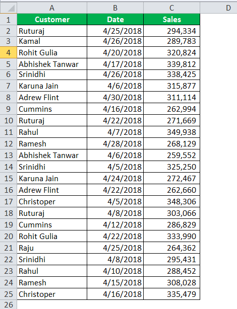
The steps to count the unique excel values by using the SUM and COUNTIF functions of Excel are listed as follows:

Step 1: Enter the following formula in cell E3.

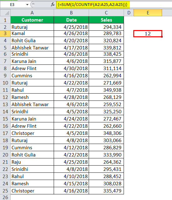
Step 2: Press the keys “Ctrl+Shift+Enter” together. This is because the given formula is an array formula. On pressing the CSE (Ctrl+Shift+Enter) keys, the curly braces appear at the beginning and end of the formula, as shown in the following image.

Note: An array formula is always completed by pressing the CSE keys. Even after editing an array formula, the CSE keys must be pressed to save the changes made. An array formula cannot be applied to merged cells.

Step 3: Once the CSE keys are pressed, the output appears in cell E3. This is shown in the following image. Hence, there are 12 distinct values in column A. In other words, the organization sold to 12 different customers in April 2018.

Explanation of the formula: The formula entered in step 1 has three parts, namely, the COUNTIF function, “1/,” and the SUM function. These are shown in the following image.

Ignore the arrows of parts 2 and 1, which are slightly misplaced in the following image.

In this formula, the COUNTIF function is processed first as it is the innermost function. Thereafter, “1/” and the SUM function are processed. The entire formula works as follows:

a. The COUNTIF function is supplied a single range (A2:A25) twice. This tells the function to count the number of times a value appears in this range. Since there are 24 values in this range, the COUNTIF function returns an array of 24 values. These are shown in the following image.

So, the first 3 implies that the name “Ruturaj” appears thrice in the range A2:A25. Likewise, the following 1 implies that the name “Kamal” appears once in this range.

b. Next, the number 1 is divided by all the values returned in the preceding array. The output is again an array of 24 values. These are shown in the following image.

Since “Ruturaj” appears thrice (in A2:A25), the value 3 divided by 1 returns 0.33. Likewise, “Kamal” appears once, so 1 divided by 1 is equal to 1. Therefore, all values that appear once in the stated range (A2:A25) return 1. The values that return a decimal number have more than one occurrence.

c. Then, the SUM function sums the values returned in the preceding array. Note that if a value appears thrice in the stated range, 0.33 (1/3=0.33) appears thrice. So, 0.33+0.33+0.33 is equal to 1. Likewise, if a value appears twice in the range A2:A25, 0.5 (1/2=0.5) appears twice. So, 0.5+0.5 is equal to 1. In this way, the sum of all occurrences of a value is always equal to 1. Therefore, the SUM function returns the total of all the different values in the range A2:A25.

Hence, the count of unique excel values (in the range A2:A25) is 12. This 12 is the sum of two unique values (Kamal and Raju) and the first occurrence of ten duplicate values (Ruturaj, Rohit Gulia, Abhishek Tanwar, Srinidhi, Karuna Jain, Andrew Flint, Cummins, Rahul, Ramesh, and Christoper).

Note: To view the array of values returned by the COUNTIF function in pointer “a,” follow the listed steps:

Select cell E3 containing the formula.
Double-click within the selected cell or press the key F2. This helps enter the Edit mode.
Select the COUNTIF part of the formula, i.e., “COUNTIF(A2:A25,A2:A25).”
Press the key F9.

Likewise, to view the array of pointer “b,” select cell E3 and double click within the selected cell. Next, select the part “1/COUNTIF(A2:A25,A2:A25)” and press F9.

To exit the Edit mode, press the escape (Esc) key.

Example #2–Count Unique Excel Values by Using the SUMPRODUCT and COUNTIF Functions

The following image shows the dataset of example #1. Count the distinct values of column A with the help of the SUMPRODUCT and the COUNTIF functions of Excel.

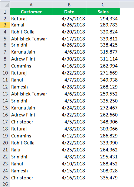
The steps to count the distinct values by using the SUMPRODUCT and COUNTIF functions are listed as follows:

Step 1: Enter the following formula in cell E6.

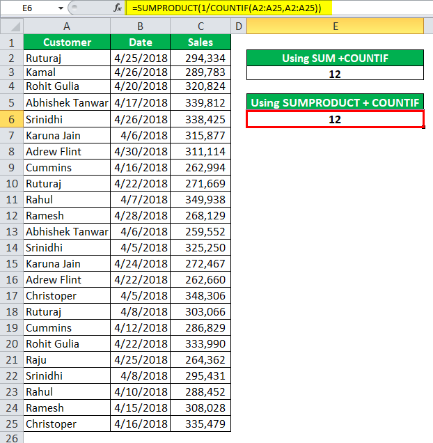
Step 2: Press the “Enter” key. The output appears in cell E6, as shown in the following image. So, there are 12 distinct values in the range A2:A25.

Notice that the output of the SUM and COUNTIF (example #1) is the same as that of the SUMPRODUCT and COUNTIF (example #2). Hence, since the outputs are the same, one can choose either of the two formulas based on convenience.

Explanation of the formula: The formula given in step 1 (of this example) works exactly the same way the formula of example #1 works. The only difference between the formulas of examples #1 and #2 is the usage of the CSE keys in the former and the usage of the “Enter” key in the latter.

In the current formula, the COUNTIF function and the division by 1 return the same array as that of pointers “a” and “b” of example #1. Being a single array, the SUMPRODUCT sums the values of this array. The output is 12. So, this 12 consists of two unique values and the first occurrences of ten duplicate values.

Note 1: For the detailed working of the current formula, refer to the “explanation of the formula” given at the end of example #1.

Note 2: To see the complete array values returned by the COUNTIF and “1/” part, one can select these parts and press the F9 key. For more details, refer to the note at the end of example #1.

Example #3–Count Unique Excel Values by Excluding the Empty Cells of the Range

Working on the dataset of example #1, we have inserted row 10 as a blank row. As a result, the formulas of examples #1 and #2 show a “#DIV/0!” error in cells E3 and E6. This error is displayed when a number is divided by zero (or an empty cell) in Excel.

Count the number of distinct values of column A by excluding the empty cell A10. Use the following functions of Excel:

SUM and COUNTIF functions
SUMPRODUCT and COUNTIF functions

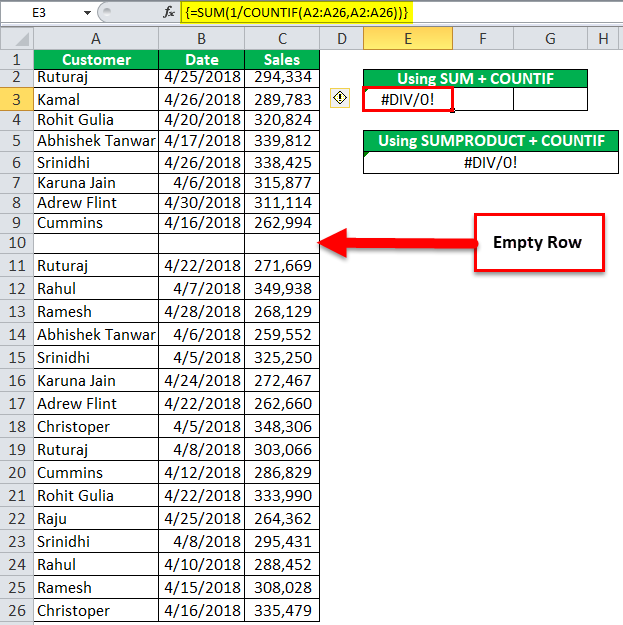
The steps to count the distinct values by excluding the empty cell are listed as follows:

Step 1: Enter the following formulas (without the beginning and ending double quotation marks) in cells E3 and E6 respectively.

“=SUM(1/COUNTIF(A2:A26,A2:A26&“”))-1”

“=SUMPRODUCT(1/COUNTIF(A2:A26,A2:A26&“”))-1”

Step 2: Press the CSE keys (Ctrl+Shift+Enter) after entering the SUM and COUNTIF formula. Press the “Enter” key after entering the SUMPRODUCT and COUNTIF formula.

The outputs of both the formulas are shown in the following image. Notice that in this image, the SUM and COUNTIF formula is displayed (in curly braces) in the formula bar.

Hence, the output of both formulas is 12. This implies that there are 12 distinct values in column A. The empty cell A10 is excluded from this count.

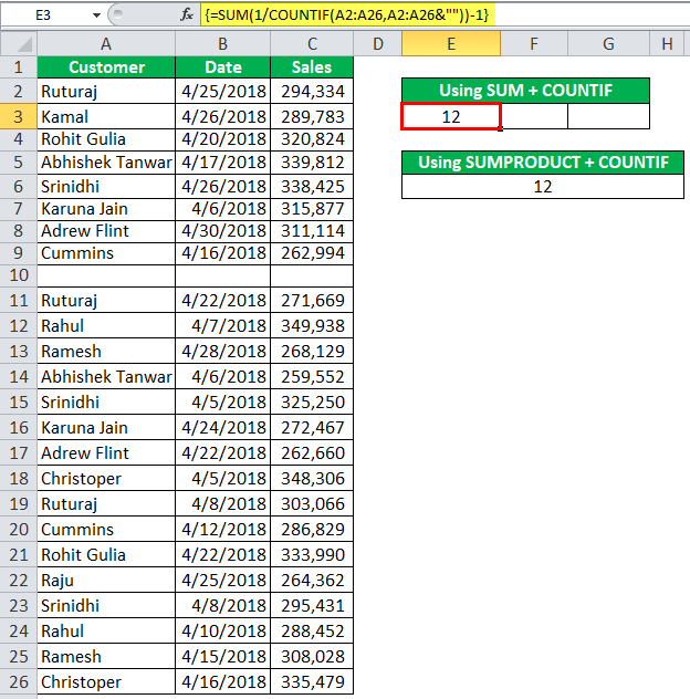
Explanation of the formulas: The preceding two formulas work as follows:

a. The COUNTIF function is instructed to count the non-blank cells within the range A2:A26. Since the ampersand operator (&) along with an empty string (“”) is supplied to the COUNTIF function, it treats the empty cell A10 as a unique value. So, the COUNTIF returns the following array of values:

{3;1;2;2;3;2;2;2;1;3;2;2;2;3;2;2;2;3;2;2;1;3;2;2;2}

b. Next, the values of the preceding array are divided by 1. This division returns the following array of values:

{0.333333333333333;1;0.5;0.5;0.333333333333333;0.5;0.5;0.5;1;0.333333333333333; 0.5;0.5;0.5;0.333333333333333;0.5;0.5;0.5;0.333333333333333;0.5;0.5;1;0.333333333333333;0.5;0.5;0.5}

c. At last, the single array is summed up by the SUM or the SUMPRODUCT functions. This returns 13 as the sum. From this sum, 1 is subtracted to exclude the empty cell from the count. So, the final output is 12.

Hence, Excel returns the same output irrespective of the formula used. Notice that in this example, the COUNTIF returned 1 for the single empty cell A10.

Likewise, had there been two empty cells in the range A2:A26, the COUNTIF would have returned 2 at two places in the array. For three empty cells, the COUNTIF would have returned 3 at three places in the array. So, the sum of all occurrences of empty cells is always equal to 1.

Therefore, the given two formulas would have returned the correct output even if there had been more than one empty cell in the supplied range.

Note: To view the array of values in pointers “a” or “b,” select the parts “COUNTIF(A2:A26,A2:A26&“”)” or “1/COUNTIF(A2:A26,A2:A26&“”)” of the formula. Next, press the key F9.

Frequently Asked Questions

1. Define unique values and state the formula for counting them in Excel.

Unique values are those that appear in a list of items only once. The formula for counting unique values in Excel is stated as follows:

“=SUM(IF(COUNTIF(range,range)=1,1,0))”

This formula works as follows:

a. The COUNTIF function is supplied with a single range twice. It counts the number of values that appear only once in the stated range. It returns an array of values.
b. The IF function considers the argument “COUNTIF(range,range)=1” as the logical test. If the COUNTIF returns 1, the IF function also returns 1 (value_if_true). However, if the COUNTIF returns a value other than 1, the IF function returns 0 (value_if_false). All ones returned by the IF function are unique values and all zeroes are duplicate values.
c. The SUM function sums the single array of ones and zeroes returned by the IF function.

The final output is the count of the unique values of the list of Excel.

Note 1: The given formula is an array formula. So, ensure that the CSE (Ctrl+Shift+Enter) keys are pressed after entering the formula in Excel. Exclude the beginning and ending double quotation marks while entering the formula in Excel.

Note 2: To extract the unique values, the duplicates need to be removed from the list.

2. Define distinct values and state the formula for counting them in Excel.

Distinct values are all the different values of a list of items. So, distinct values are the unique values plus the first occurrences of duplicate values.

To count the distinct values in Excel, either of the following formulas can be used (without the beginning and ending double quotation marks):
• “=SUM(1/COUNTIF(range,range))”
• “=SUMPRODUCT(1/COUNTIF(range,range))”

The only difference between the two formulas is that the former is completed with the CSE (Ctrl+Shift+Enter) keys, while the latter is completed with the “Enter” key.

Note: For more details on the working of the preceding formulas, refer to examples #1 and #2 of this article. For counting distinct values by excluding the empty cells, refer to example #3 of this article.

3. How to count the unique and distinct values by using the COUNTIFS function of Excel?

The formula for counting the unique rows of ranges A2:A12 and B2:B12 is stated as follows:

“=SUM(IF(COUNTIFS(A2:A12,A2:A12,B2:B12,B2:B12)=1,1,0))”

The formula for counting the distinct rows of ranges A2:A12 and B2:B12 is stated as follows:

“=SUM(1/COUNTIFS(A2:A12,A2:A12,B2:B12,B2:B12))”

Both the COUNTIFS formulas work similar to their COUNTIF counterparts. The benefit of using the COUNTIFS function is that it allows checking multiple columns for unique or distinct values.

Note: A row will be counted by the two formulas only if the cells in both columns A and B are unique (or distinct). Further, both the stated formulas are array formulas. So, do press the CSE (Ctrl+Shift+Enter) keys to complete these formulas.