Correlation Matrix in Excel

Correlation assesses the dependency of one variable on the other. It shows how the impact of an increase or a decrease in one variable affects the other. In multiple correlation, more than two variables are studied at the same time.

The correlation coefficient can be positive (+1), negative (-1), or zero (0).

• Positive correlation: The correlation coefficient is “+1,” which implies that the two variables move in the same direction.
• Negative correlation: The correlation coefficient is “-1,” which implies that the two variables move in opposite directions.
• Zero correlation: The correlation coefficient is “0,” which implies that the two variables are not dependent on each other.

The features of correlation are stated as follows:

• The correlation shows the cause and effect relationship between several factors.
• The closer the correlation coefficient is to “+1” or “-1,” the stronger the relationship between the two variables.
• The presence of the correlation coefficient does not indicate that there is a relation between the variables.
• While computing the correlation, any number of variables can be added to the existing data with a corresponding adjustment to the range.

Note: The correlation coefficient is calculated with the help of the CORREL function of Excel.

Let us consider some examples to understand the creation of a correlation matrix in Excel.

Correlation Matrix With Analysis Toolpak

Below are the steps to add Analysis Toolpak in MS Excel

The Analysis Toolpak is an add-in option available under the Data tab of the Excel ribbon. The steps to add this option are listed as follows:

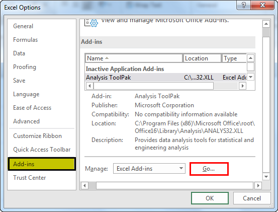
• Click on “file” and select “options.”

• In “options,” select the “add-ins” button. Click on “go” displayed next to the dropdown of “manage.”

• Select the check box for Analysis Toolpak and click “Ok.”

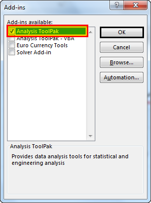
• The Toolpak gets added to the Data tab as “data analysis” (under the “analysis” section).

Steps to Create Correlation Matrix using Analysis Toolpak

Correlation Matrix for Multiple Variables

Let us consider another example.

The steps to create a correlation matrix for multiple variables are listed as follows:

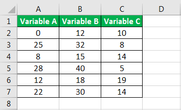
• In an Excel sheet, enter the data for multiple variables, as shown in the following image.

• Click on “data analysis.”

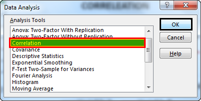
• Select “correlation” in the “data analysis” pop-up window. Click “Ok.”

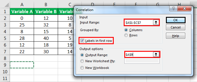
• The “correlation” pop-up window appears. In this, perform the following tasks:
  • Select the data range (A1:C7) of the three variables in the “input range” field.
  • Select the check box for “labels in first row” because the first row contains labels.
  • In “output range,” enter the cell number where you want the resulting table.
  • Click “Ok.”

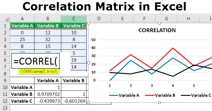
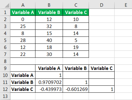
• For the three variables A, B, and C, the correlation matrix appears in the range A9:D12.

The correlation matrix consists of the variable label in the first column (or row) and the correlation coefficients in the subsequent columns (or rows). To understand the matrix, the correlation coefficient corresponding to the intersection of the row and column must be read.

The findings of the table (in the previous example) are listed as follows:

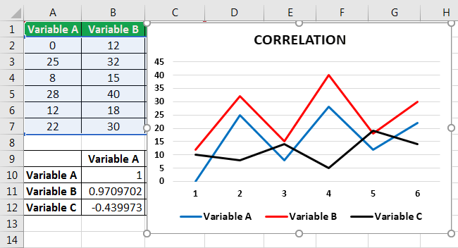
• The correlation coefficient for variables A and B is 0.97. This implies that these variables are positively correlated.
• The correlation coefficient for variables B and C is -0.6. This implies that these variables are negatively correlated.
• The correlation coefficient for variables A and C is -0.43. This implies that these variables are not correlated.

The relation between the variables A, B, and C is shown in the following graph.