Table Of Contents
What Is Convert Numbers To Text In Excel?
Convert Numbers to Text in Excel is a feature to convert the numeric value to text values using the TEXT function in Excel and the Format Cells option.
The Excel Convert Numbers to Text is useful because some datasets may contain long dates, alpha-numeric values, or text strings saved in numeric formats. In such scenarios, to get the accurate output, we must convert the format first and then execute the formulas.
Key Takeaways
- The Convert Numbers to Text in Excel changes the digits to text strings.
- We can open the Format Cells window using the following methods, namely,
- Use the shortcut keys to “Ctrl+1” in windows, and “COMMAND+1” in Mac.Select the “Home” tab - go to the “Number” group - click the “Number Format” option drop-down - click the “More Number Formats…” option.
- Right-click on any cell - select the “Format Cells…” option.
- We can use some functions to convert numbers, such as Text(), Exact(), and Sumproduct(), along with Isnumber() and Find() functions.
How To Convert Numbers To Text In Excel?
We can Convert Numbers to Text In Excel using two different methods, namely:
- Method #1 – Use the “TEXT” function in Excel.
- Method #2 – Use the “Format Cells” option.
#Method 1 - Convert Numbers to Text using Excel TEXT Function
The TEXT function converts numbers formatted as numbers to text in the specified format in Excel.
The TEXT Formula in Excel syntax is,

The TEXT Formula in Excel arguments are,
- value: The value for which text formatting is required. It can be any number entered directly or as a cell reference. It can also be a mathematical operation or a date. We can also specify TODAY() or MONTH() etc., in the value.
- format_code: The formatting code is necessary for a number. The various format_code available in Excel are always given in a double quotation mark. For example, you can use “0” to specify an integer with zero decimal place, “0.000” to specify three decimal places, “0000” to add leading zeros, etc. We can also select percentages, scientific notations, currency, degrees, and date formats in the TEXT function, such as “0.00%”, “$0”, “##0° 00′ 00″”, “DD/MM/YYYY”.
Returns -
The function returns a number as text in the specified format.
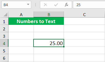
Suppose you have cell B4 containing the number 25.00 and formatted as a number. You want to convert numbers to text format.
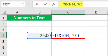
You may give the TEXT formula as: =TEXT(B4,“0”)
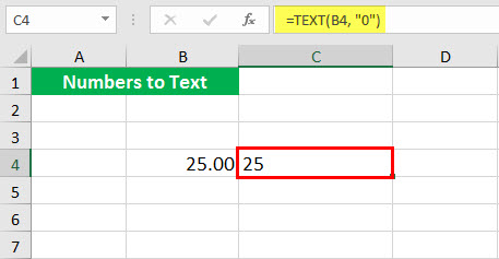
It will return the number in text format.
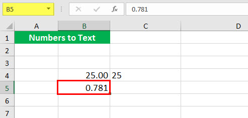
Suppose we have a number as 0.781 in cell B5. We want to convert this number to a percentage.
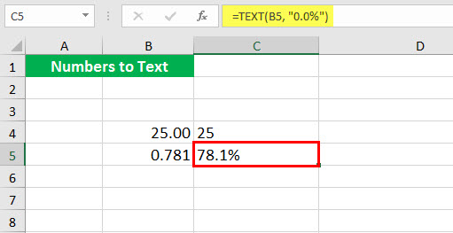
We can use the following TEXT formula: =TEXT(B5,“0.0%”)
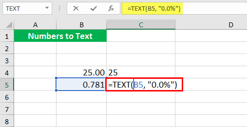
As a result, it will return 78.1% as a TEXT format.
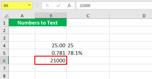
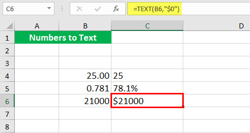
Suppose we have a number 21,000 in cell B6. We want to display the number as currency in the dollar.
To do this, we can use the TEXT Formula in Excel:
= TEXT (B6, “$0”)
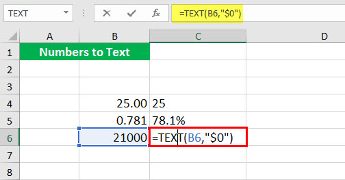
It will return $21000.
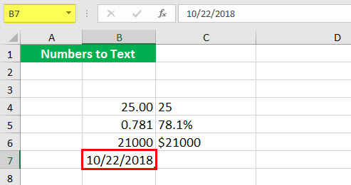
Suppose we have a date 10/22/2018 in cell B7, and we have to convert the date to another format.
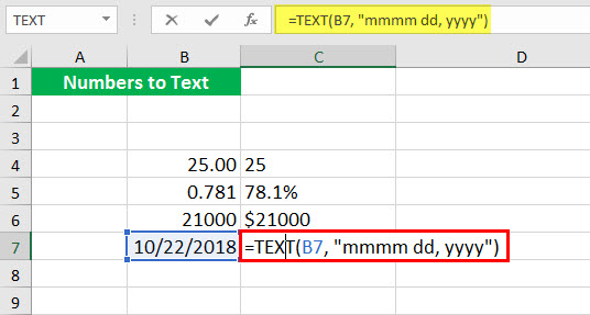
We can use the TEXT formula: = TEXT (B7, “mmmm dd, yyyy”)
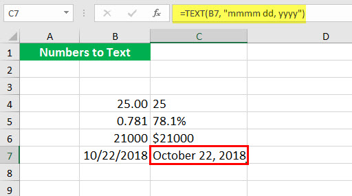
It will return the date specified, i.e., October 22, 2018, as shown below.
#Method 2 - Convert Numbers to Text using Excel Format Cell Option
Besides using the TEXT function, we can also use the Format Cell option to Convert Numbers to Text in Excel.
Suppose we have a number 25 in cell B11. We want to convert numbers to text.
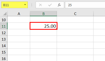
To do so, we can press “CTRL + 1″ (or COMMAND + 1 on Mac). As a result, a dialog box may appear, similar to the one shown below.
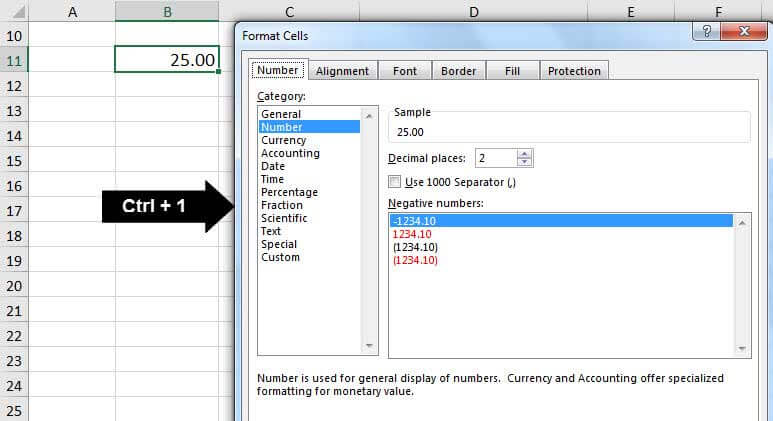
It mentions that the cell is currently formatted as a number. Now, we must select the “Text” option in the category.
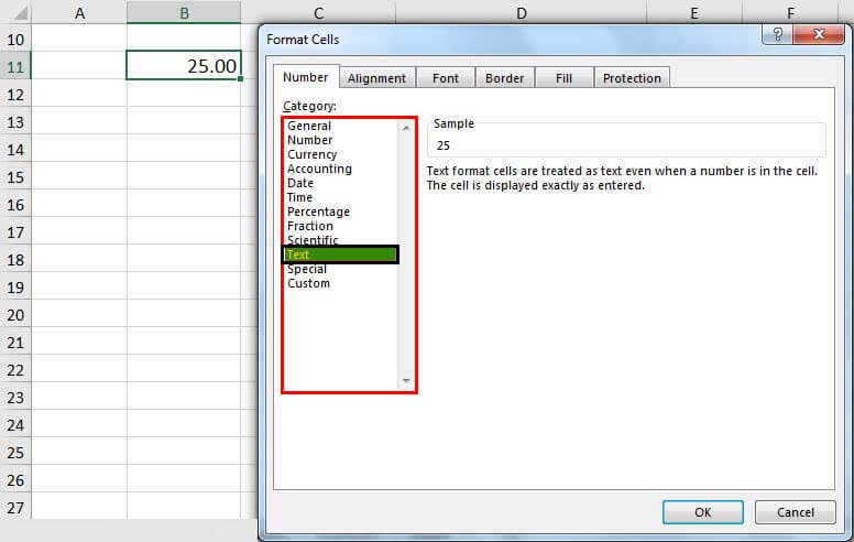
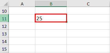
And click “OK”. We notice that the number has been formatted as “Text” now.
Similarly, we can change the formatting to a percentage, date, scientific notation in excel, etc.
Suppose we want to convert cell B13 to percentage format.
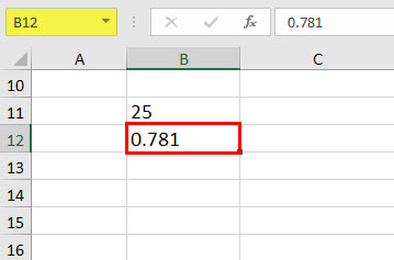
We must select the cell and press “CTRL + 1” (or COMMAND + 1 for Mac), and select “Percentage.”
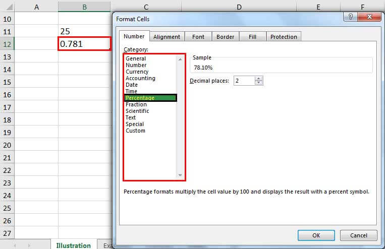
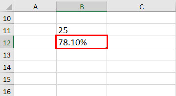
Then, click “OK.”
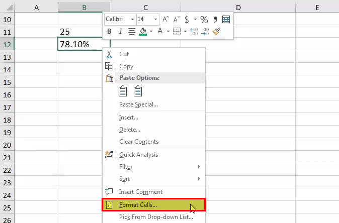
Instead of pressing “CTRL + 1” (or COMMAND + 1 in Mac), we can also right-click on the selected cell and then click “Format Cells,” as shown below.
As shown in the above steps, we can select the “Text” option in the category and click “OK.”
Examples - Where can you Convert Numbers to Text in Excel?
We will consider some examples to Convert Numbers to Text In Excel using each methods with an example.
Example #1
Suppose we have the start and end timings of different sessions held in the upcoming workshop organized by your company, as shown below. We are supposed to merge the two times, creating a range (time duration).
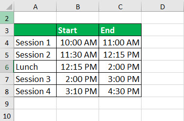
We first need to convert the time into “Text” format and then merge them to get a time range. For the first session, we can use the following TEXT formula:
= TEXT( B4, “hh:mm” ) & ( ” – ” ) & TEXT( C4, “hh:mm” ) & ( ” Hrs” )
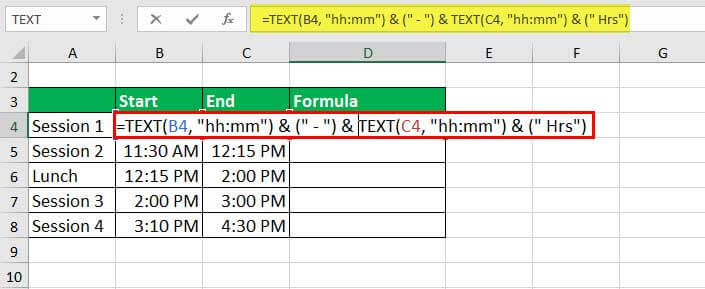
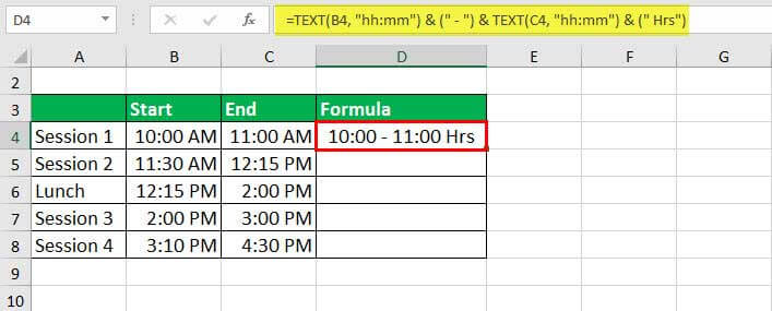
It will return the time range for the 1st session.
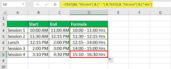
Now, we can drag it to the rest of the cells to get the range for the rest of the cells.
Now, let us see the syntax in detail:
TEXT( B4, “hh:mm” ) & ( ” – ” ) & TEXT( C4, “hh:mm” ) & ( “Hrs” )
- TEXT( B4, “hh:mm”), will convert the given time in cell B4 to text in an hour: minute format (24 hours). Similarly, TEXT( C4, “hh:mm”), will convert the given time in cell C4 to an hour: minute format.
- & (“-” ) &, will add “-” in between the two times, thus, creating a range.
- & (“Hrs”), it will add the text Hrs at the end.
Similarly, we can also create a range of dates by modifying this syntax.
Example #2
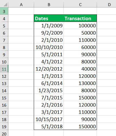
Suppose we have data for certain transactions accomplished in the past few years. Of those transactions, we want to know how many transactions were made during a particular month of a specific year and the total transaction amount. Therefore, the transaction data is given the cells B5: C19, as shown below.
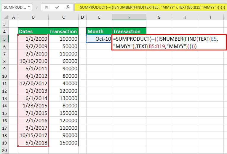
The month and year to look for are given in cell E5. To search the number of transactions held in the given month, we can use the SUMPRODUCT formula:
=SUMPRODUCT(–((ISNUMBER(FIND(TEXT(E5, “MMYY”),TEXT(B5:B19, “MMYY”))))))
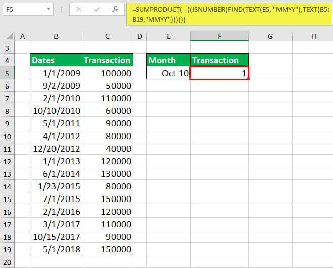
And press the “Enter” key.
Now, to identify the total transaction amount during that period, we can use the following SUMPRODUCT Formula:
=SUMPRODUCT(– (EXACT( TEXT(E5, “mmyy”), TEXT( B5:B19, “mmyy”)) ), C5:C19)
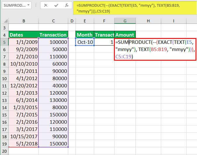
It will return to 60000.
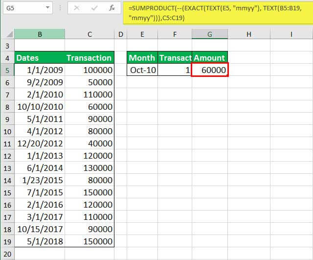
In both cases, the date given in cell E5 is first converted to “MMYY” format, and the dates given in cells B5:B19 are also converted to the same format and then matched. In the first case, wherever there is a match, it will return “TRUE” or “FALSE,” making an array. This array is then converted to numbers using ISNUMBER, returning an array of 0 and 1. The SUMPRODUCT function will then count the number of 1 (i.e., TRUE, i.e., where we found the match), returning the number of transactions. The EXACT function will get the corresponding value wherever there is a match in the latter case. The SUMPRODUCT function will then sum the total transactions where we obtained a match.
Important Things To Note
- We must avoid losing any number by changing the data into text. For example, if the number starts with “0”, we may lose this initial zero when we copy-paste it into another cell.
- To retain the numbers as text or avoid getting errors when we copy-paste them into another sheet, we can first paste the copied data in a notepad, then copy from there and paste it into the workbook.

