Convert Date to Text in Excel

When we work in Excel often, we deal with numbers, text, and date format. Excel completely works on numbers. It will reflect the values based on the formatting you give. For example, the date and Time in excel are stored as numbers and converted to readable values based on the formatting.

Look at the below example; the value in cell A1 is 43388. But, if we format it to date, it will show us the value as 15-10-2018.

First, we must right-click on the cell and select the "Format Cells" option.

Then, we need to select the date option as shown below.

Now, the result will be as below.

So, Excel will reflect the numbers based on the formatting we apply.

Now, let us see some examples of converting dates to text in Excel.

When we need to convert Date to Text in Excel, we need to use the TEXT function in Excel. As mentioned, time and date in Excel are stored as numbers. However, sometimes we may require showing it as the text string. In such cases, we can use the TEXT function

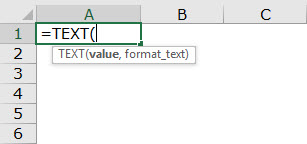
• TEXT function consists of VALUE & FORMAT_TEXT.
• VALUE: It is the value we need to convert. It is simply the targeted cell. That could be a number, a reference cell that contains a number.
• FORMAT_TEXT: The format we need to provide to the cell, i.e., the targeted cell.

There are multiple date formats available in Excel. The below table will provide a better idea about the different formats and results.

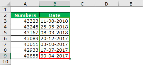
We have the below values from cell A2 to A10 and convert them to the Date from B2 to B10.

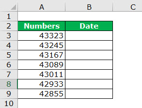
To convert them to date format, in cell B2 write the below formula.

=TEXT(A3,"dd-mm-yyyy")

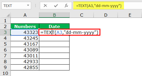
Press enter and drag the formula

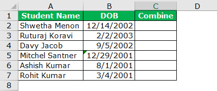
Take the below data and join the two columns (A2 & B2) together. For example, get the result as Shwetha Menon's Birthdate is 14 Dec 2002.

Step 1:

If we do not like formulas in Excel to convert the date to text format, we can use the TEXT TO COLUMN OPTION. Assume we have data from cells A2 to A8.

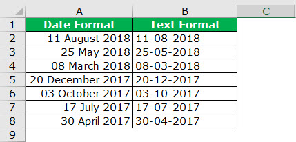
Now, we need to convert it into text format.

Step 1: We must first select the whole column that we want to convert.

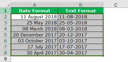
Step 2: Then, we must go to Data > Convert Text to Columns Wizard in Excel.

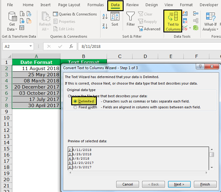
Step 3: We must ensure that the delimiter is selected and click the "Next" button.

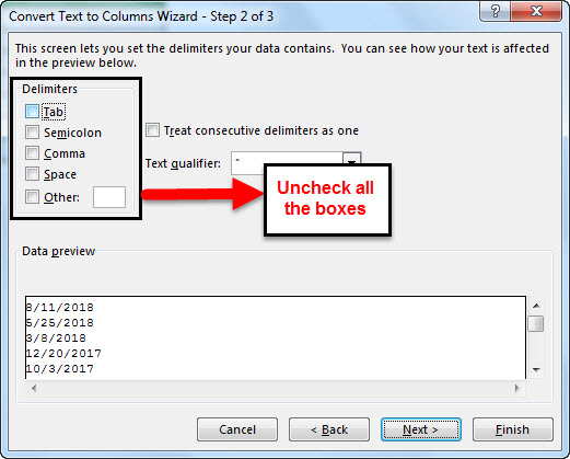
Step 4: Now, the pop-up below will open and uncheck all the boxes and click the "Next" button.

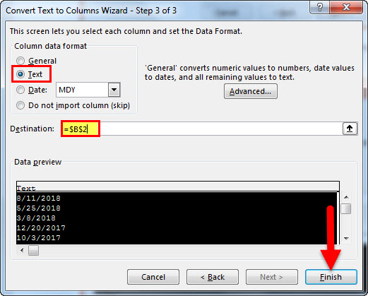
Step 5: We must select the "TEXT" option from the next dialog box. Then, we need to mention the destination cell as =$B$2 and click "Finish."

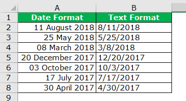
Step 6: As a result, it will instantly convert into text format..

We must use the formula method to convert the number to a date format. Assume we have the below data in our Excel file.

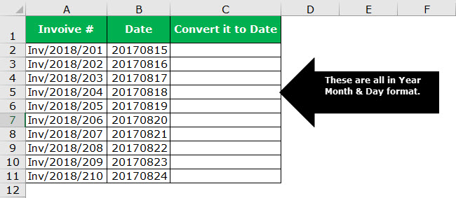
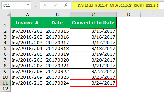
Formulas you need to know to convert them to YYYY-MM-DD are DATE, LEFT, RIGHT & MID functions. Moreover, the formula is.

Date: Date Function in Excel formats it into Year-Month-Day format.

Left: LEFT Function in Excel will take the first portion for year format. It takes 4 first 4 characters in year format.

Mid: MID Function will take the middle part of the data for month format. It takes the middle 2 characters for a month format.

Right: RIGHT Function in Excel will take the last part for Day format. Takes the last 2 characters for Day format.

Now, we must go ahead and apply the formula to get the date format.

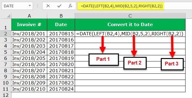
Now, let us elaborate on each part.

Part 1: LEFT (B2, 4) this means, in cell B2, take the first four characters. i.e., 2017

Part 2: MID (B2, 5, 2) this means, in cell B2, starting from 5^th character, select two characters. i.e., 08.

Part 3: RIGHT (B2, 2) this means, in cell B2 from the right side, select two characters. i.e., 15

The Date function will combine all these and give you the value below. Next, drag and drop the formula for the remaining cells.