Table Of Contents
What Is Conditional Formatting In Pivot Table?
Conditional Formatting is a feature in Excel that helps users to highlight desired cells or rows based on the rule we set or the formula we input. Conditional Formatting in Pivot Table is the same, except it highlights the required data in the generated Pivot Table.
Key Takeaways
- Conditional Formatting in Pivot Table helps us highlight the desired data in the Pivot table that is generated. It’s important to understand these two features individually.
- Conditional Formatting highlights specific words, or rows as per the set rule. Pivot Table is a new table generated for a dataset or a cell range that has automatic filters for easy display of data.
- Ensure to refresh the Pivot Table when data modification is done because the Conditional Formatting may not work as it is set for a fixed dataset.
- We can also create Pivot Table Slicers linked to the existing Pivot Table.
Easy Steps To Apply Conditional Formatting In The Pivot Table
The steps to apply Conditional Formatting in the pivot table are,
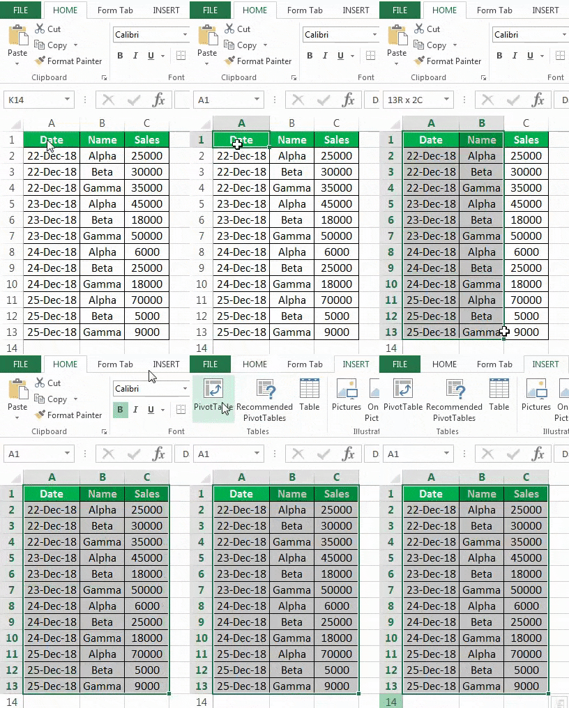
First, we must select the data. Then, in the “Insert” Tab, click on “PivotTable”.

As a result, the “Create PivotTable” dialog box appears, as shown below.

Next, we must insert the pivot table in a new worksheet by clicking “OK”. Currently, a pivot table is blank. Next, we need to bring in the values.

Then, drag down the “Date” in the “Rows” Label, “Name” in the “Column,” and “Sales” in “Values.”

As a result, the pivot table will look like the one below.

To apply Conditional Formatting in the pivot table, first, we must select the column to format. In this example, select “Grand Total Column”. Then, in the “Home” Tab in the “Styles” section, click on the “Conditional Formatting” option drop-down to open the available options, then click the “New Rule” option, as shown below.

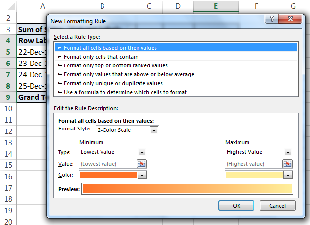
As a result, the “New Formatting Rule” dialog box will pop up.

There are a variety of rules to be applied in the pivot table. For example, we will select “Format only cells that contain”, and we can see another dialog box in the same window.

Next, we must insert any value in the “Cell Value” section. In this case, we have mentioned a range from 70000 to 90000.

Then, click the “Format” option at the bottom.

Next, we must select the type of formatting we want. For example, we have chosen a color (red color) from the “Fill” section.

After that, click “OK”, and once again “OK” to close the “Formatting Rule” dialog box.

And the pivot table is formatted in red with the values between 70000-90000, as shown above.
Example
We will consider an example for Conditional Formatting in Pivot Table.
We have data for a newly launched canteen, and we have the records for the number of products sold in each of the five months – Jan, Feb, March, April, and May.

The steps to insert a pivot table in this data are:
- Step 1: We must select the data. Then, in the “Insert” Tab, click on “PivotTable”.

- Step 2: Then, insert the pivot table in a new worksheet by clicking “OK”.

- Step 3: Drag down the “Product” in the “Row” label and “Months” in the “Value” fields.

- The pivot table will look as shown below.

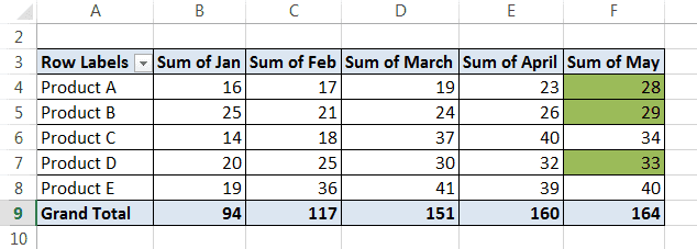
- Step 4: Our motive is to highlight those cells with the highest number of products sold in each row. For that, we must select any cell in the pivot table. Then, click on “Conditional Formatting” and click “New Rule”.

- Step 5: In the first option, apply a rule to select the third option.

- Step 6: Now, select the third option of “Format only top and bottom ranked values” in “Rule type”.

- Step 7: In “Edit the Rule Description”, we must enter 1 in the input box, and from the drop-down menu, select “each Column Group”, as shown below.

- Step 8: Then, we must click on the “Format”.

- Step 9: Select “Green Color” in the “Fill” section. And click on “OK”

- Step 10: Again, click on “OK” to close the formatting rule dialog box.

The above formatting compared the value in the column. If we want the formatting in the rows, we can select each row group.
Rules For Conditional Formatting in Pivot Table
In the “Home” tab under the “Styles” section, there is a button for “Conditional Formatting”. We can insert a new rule as per our requirements.
There are various rules for Conditional Formatting, as follows:
- Format Cells based on their values.
- Format cells that only contain specific data.
- Format only top and bottom ranked values.
- Format only values that are above or below average.
- Use a formula to determine which cells to format.
Important Things To Note
- We must select rules as per requirement.
- For example, when Conditional Formatting is applied to a block of cells, formatting is applied to only those specific cells.
- Any change in data may represent the wrong illustration in Conditional Formatting in Pivot Tables.

