Conditional Formatting For Dates

The Conditional Formatting for Dates is a feature where we highlight different dates in a dataset, such as due dates, weekends, holidays, date range, etc. The best way to do so is by using the “Conditional Formatting” by creating a New Rule, or by entering a simple formula. We can also use the “Format Painter” option available in Excel.

For example, in a month, we can highlight the weekends as shown below.

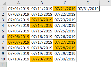
• The Conditional Formatting for Dates helps in highlighting the required dates while preparing a calendar w.r.t holidays, weekdays, weekends, important dates, etc.
• Since the formatting is for the dates, we use the TODAY and WEEKDAY functions, and also, for a date range, we use the COUNTIF function. If we must compare the dates as greater than, less than, or equal to, we can use the AND function.
• The best application for this feature is when we want to highlight dates in a calendar for the upcoming project plan, and the dates just pop up with the formatted rules.

We can use the Conditional Formatting for Dates by setting a rule to highlight the required dates using the “Conditional Formatting” option in the “Home” tab.

Using Excel Conditional Formatting for Dates, we can perform the following for a date range in excel, namely,

• Highlight Due Dates Which are Due Today.
• Highlight Weekend Dates using Conditional Formatting.
• Highlight Dates between Two Dates using Conditional Format.
• Highlight All the Holidays Dates using a Conditional Format.

Grasping these principles is essential for anyone looking to excel in this area. For those who want to take their learning to the next level, this Automated Data Entry Form Using VBA Course is designed to build on this foundation and enhance their expertise.

We will consider examples to perform the above-mentioned highlighting.

Example 1 – Highlight Due Dates which are Due Today

When you work with the accounts team, either you work in the accounts receivable team or the accounts payable team. Both teams tend to work with due dates.

• For an accounts receivable team, collecting the money on time is necessary.
• Similarly, for a payable team, it is important to payout all the payments on or before the due date to avoid consistent follow-ups from vendors.

For example, let us look at the following invoice data.

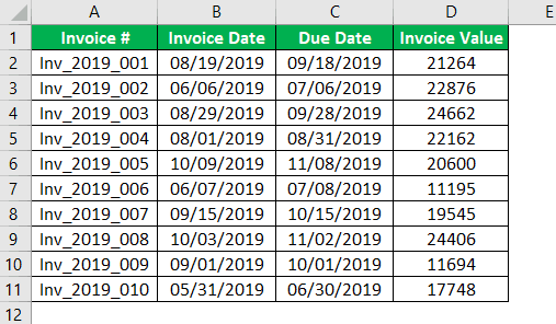
From the above, we have “Due Date” in this column. In addition, we have certain due dates over the due date, which are due today and are not yet due so far.

The steps to use Conditional Formatting to highlight dates are as follows:

1. First, select the due date column.

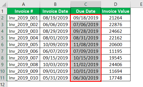
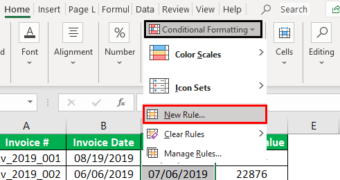
2. Then, go to Conditional Formatting, and click New Rule.

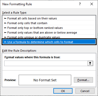
3. Now, choose “Use Formula to determine which cells to format”.

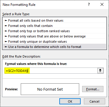
4. In the Formula section, insert the TODAY formula, shown below, to identify the due dates.

5. Now, click FORMAT, and choose the formatting color as desired.

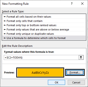
6. Now, click OK to apply the formatting.

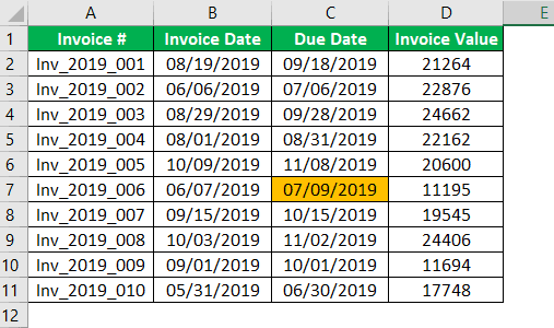
Now, let us look at the table in cell C7. It is highlighted because today’s date is “09th July 2019”, so Conditional Formatting has highlighted the due date. After all, we use the today in excel.

Similarly, we must apply to format for due dates beyond the due date. Again, we must use new Conditional Formatting, and insert the formula, as shown below.

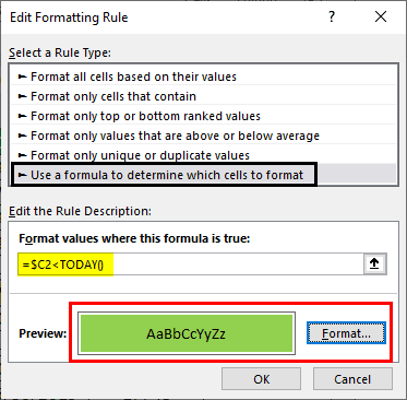
Now, click “OK”. As a result, it will highlight all the dates beyond the due date.

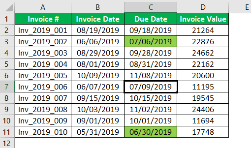
So, the dates 6th July and 30th June are beyond the dates in the table above. However, the TODAY function is a volatile formula. It keeps changing daily, and no need to worry about today’s date.

Example #2 – Highlight Weekend Dates using Conditional Formatting

We will highlight only weekend dates with all the dates available.

For example, look at the below data of dates in the entire month.

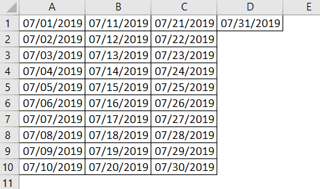
To highlight all the dates which belong to the weekend, we must follow the below steps.

In the formula section of the Conditional Formatting, insert the formula:

=WEEKDAY(A1,2)>5

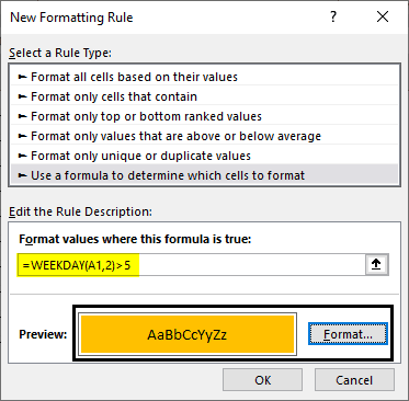
We will get the following result.

Here, we have applied the WEEKDAY in excel formula with the following syntax,

The WEEKDAY function checks all the selected cell dates and weekday numbers. For example, suppose the week starts from MONDAY (WEEKDAY(A1,2)), it will give the weekday number in the week. If the number provided by the WEEKDAY function is >5, i.e., Saturday and Sunday, it will highlight the weekend dates.

Example #3 – Highlight Dates between Two Dates using Conditional Format

For example, let us look at the below data of dates.

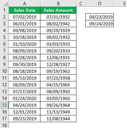
We need to identify sales dates from this sales data between 23rd April 2019 and 24th September 2019.

So, we must open the “Conditional Formatting” tab, enter the formula below, and choose the formatting as per choice.

We have applied the AND function in excel here. It will identify the dates between 23rd April 2019 to 24th September 2019 and use the formatting.

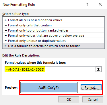
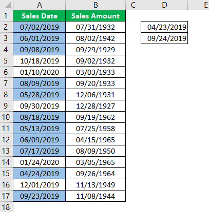
As a result, it will highlight the dates between those two dates, as shown below.

Example #4 – Highlight All the Holidays Dates using a Conditional Format

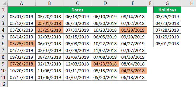
For example, we can use Conditional Formatting if we have a list of dates and want to highlight all the holiday dates.

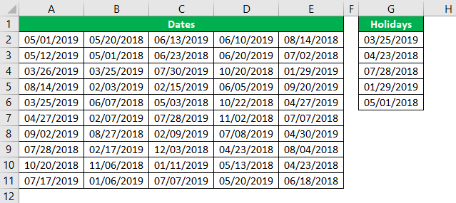
In the above list, we have dates, and also a list of holidays that we need to highlight.

So, in Conditional Formatting, we must apply the below function.

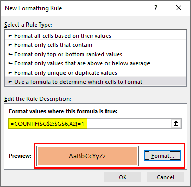
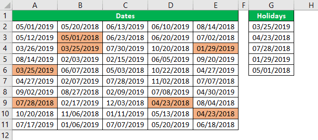
So, this will highlight all the holiday dates in the date list.

• Conditional Formatting works according to the new rule provided.
• We can format the dates that are due today, which are beyond the due date, which are yet to be due, etc.
• Using formulas in the condition, we can conduct logical tests.
• We can apply only logical tests in excel in Conditional Formatting.