Table Of Contents
How to Apply Conditional Formatting for Blank Cells?
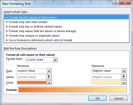
We can access the conditional formatting for blank cells from the "New Formatting Rule" of the "Conditional Formatting" tab and the cells containing blank values, the second option. In other words, it means a certain cell that does not have a value assigned to it. For example, it does not have a numeric, alphabetic, or character as a value. It is just a blank.
Examples
Example #1 - General Method to Conditional Format for Blank Cells
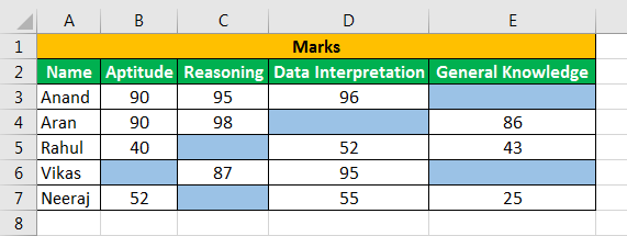
We will consider the following data given below.
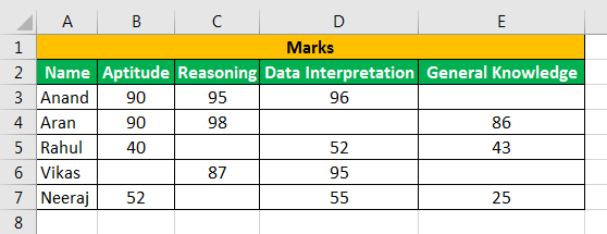
The above data shows that we have marks for five students but not for every subject. That is because some of the cells are left blank.
- We must first select the data range in which we want to use conditional formatting. In the "Home" tab, under the "Styles" section, click on "Conditional Formatting," Then, click on the "New Rule."
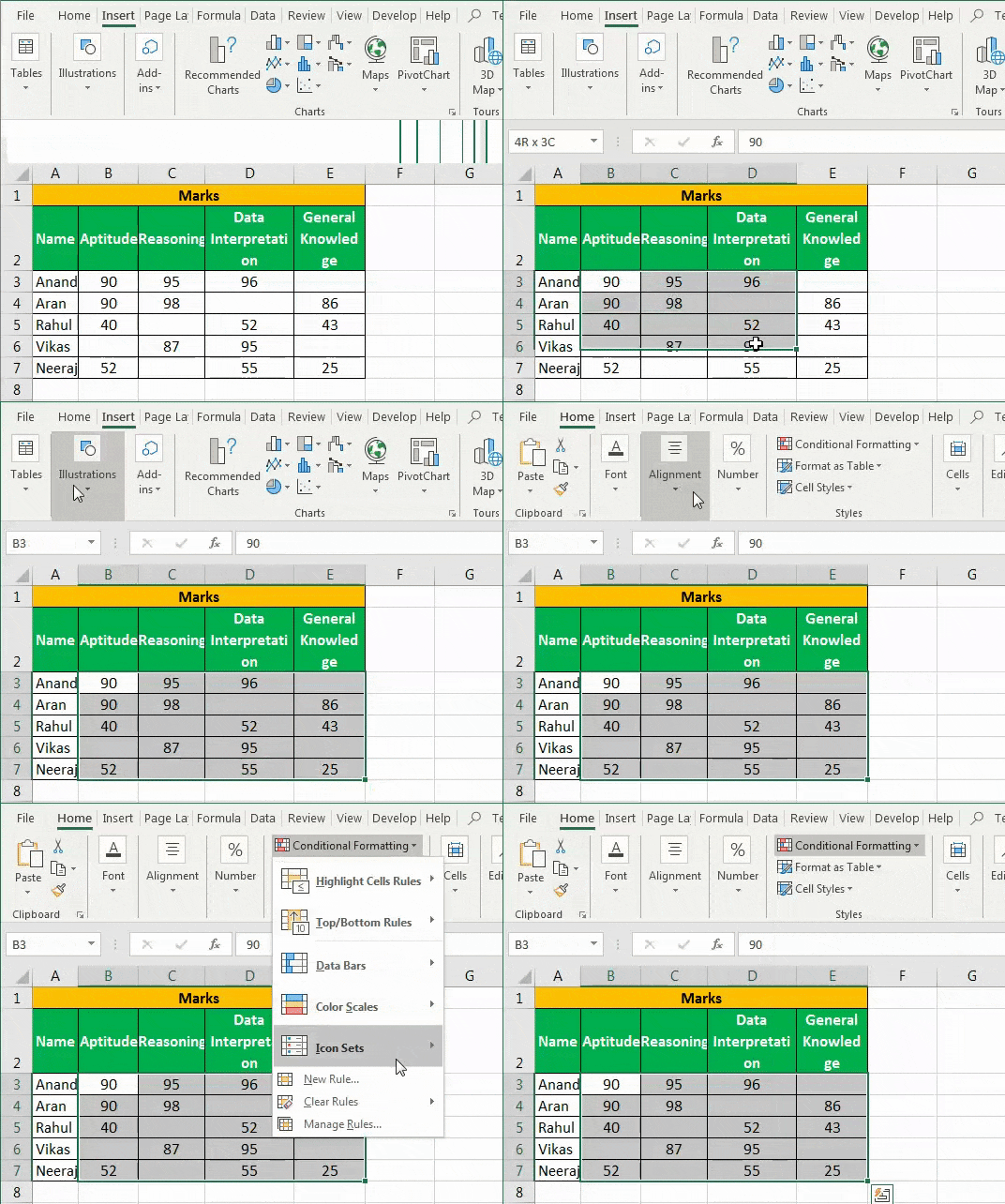
- When we click on the "New Rule," another wizard box appears, the "New Formatting Rule" tab.

- Then, we must click on the second option, "Format only cells that contain."

- Click on "Format only cells with" on the left-hand side below and select the option "Blanks."

- Click on "Format" and select any option we desire to format the cells.
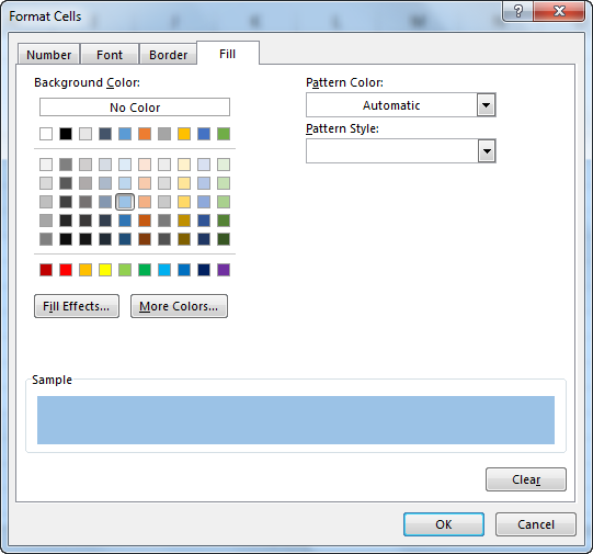
- We have selected a blue color as a formatting option. As we click on "OK," it will show the result like the one below.
Example #2 - Conditional Formatting for Blank Cells using ISBLANK Function
- Step #1 - We will repeat the same steps and go to "Conditional Formatting" in the "Styles" section under the "Home" tab.

- Step #2 - Now, we will click on "New rules" from the wizard box and then select the option on the last option from the rule types.
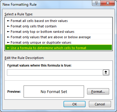
- Step #3 - In the formula box, we must insert the following formula:
ISBlank($E$3)

- Step #4 - We must click on "Format" and select the desired formatting. For instance, we have chosen the blue color this time.
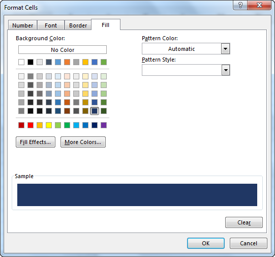
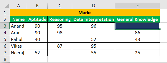
- Step #5 - Then, click on "OK." We can see that the blank cell has been identified and formatted to blue.
Things to Remember
- We can also use the ISBlank or IF function formula to format the blank cells.
- Once the cells are no longer blank, the formatting is automatically removed from them.
