Conditional Formatting Based On Another Cell Value

Last Updated :

Blog Author :

Edited by :

Reviewed by :

Table Of Contents

What Is Conditional Formatting Based On Another Cell Value?

Conditional Formatting Based on Another Cell Value is a feature where we format a cell based on the value of different cells. We can format an entire row based on a single column’s cell value. We can compare values like greater than, less than, or equal to, from another cell value to highlight the existing dataset.

How To Use Conditional Formatting Based On Another Cell Value?

We usually highlight an Excel row, column, or a cell value based on specific or multiple criterias to give various highlighting options. Here, we will see how to apply Conditional Formatting with the following cell values criteria, namely:

Criteria #1 - Text criteria
Criteria #2 - Number criteria
Criteria #3 - Multiple criteria
Criteria #4 - Different color based on multiple conditions
Criteria #5 - Where any cell is blank
Criteria #6 - Based on a drop-down selection

What Is Conditional Formatting Based On Another Cell Value?

Conditional Formatting based on another cell value helps us create a rule or a formula to compare values like greater than, less than, or equal to, from another cell value to highlight the existing dataset.
Conditional Formatting helps us highlight errors, empty or blank cells, specific words, or any symbols, alphabets, or characters in the selected cells.
We can use this feature to distinguish the required data using color coding, various border styles, etc., in a large dataset to highlight accordingly to easily understand just with a look.
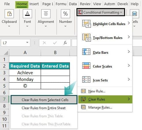
As we also saw, we can clear the set Conditional Formatting Rules for the selected data or the entire sheet too.

Example

We will consider an example for Conditional Formatting based on another cell criteria.

Below is the list of online products with different customer orders.

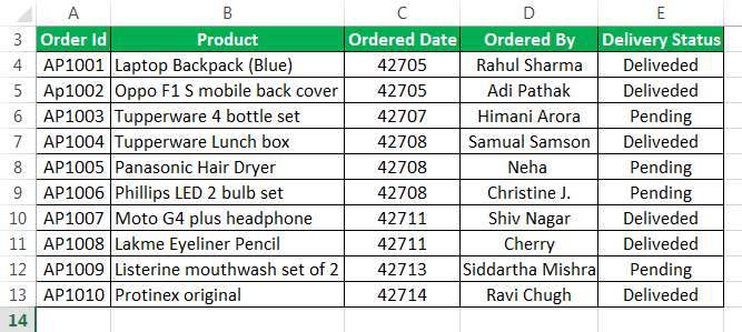
Conditional Formatting Another cell Example 1

We have to identify the records whose delivery status is pending. We want to format the “Order ID,” “Product, Ordered Date,” “Ordered By,” and “Delivery Status” based on the value in the “Delivery Status” column.

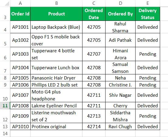
Conditional Formatting Another cell Example 1-1

We want to format the entire row based on “Delivery Status,” whose value equals “Pending.”

When we want to format a cell based on the value in a different cell, we will use a formula to define the Conditional Formatting Rule. It is an easy process to set up a formatting formula.

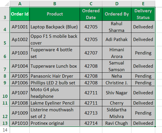
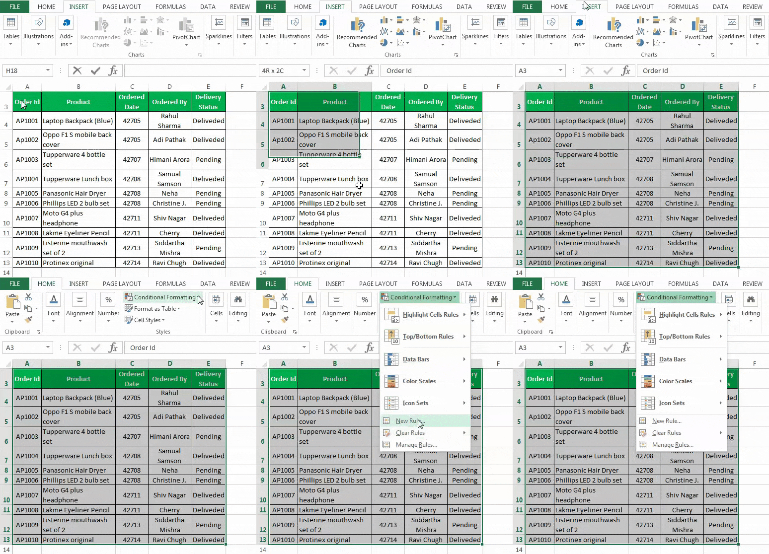
First, we must select the whole data from A3:E13, as shown below.

Conditional Formatting Another cell Example 1-2

Then, go to the “HOME” tab. Click the “Conditional Formatting.” Finally, choose the “New Rule” option.

Conditional Formatting Another cell Example 1-3

As a result, it will open a dialog box for setting a new rule, as shown below.

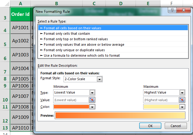
Conditional Formatting Another cell Example 1-4

This dialog box has many options, such as,

Format all cells based on their values
Format only cells that contain
Format only top or bottom ranked values.
Format only values that are above or below average
Format only unique or duplicate values
Use a formula to determine which cells to format

We must select the last option, “Use a formula to determine which cells to format.”
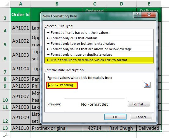
We need to set up a formatting formula to return a “True” or “False” value.
If the value is true, it will apply the desired formatting in excel. Otherwise, the formatting is not used.
In the formula input box, enter the formula =$E3=“Pending”, as shown below.

First, we must click the “Format” button. Then, a “Format Cells” dialog box will appear. Next, set the color to highlight the row. Finally, you may refer to the below screenshot.

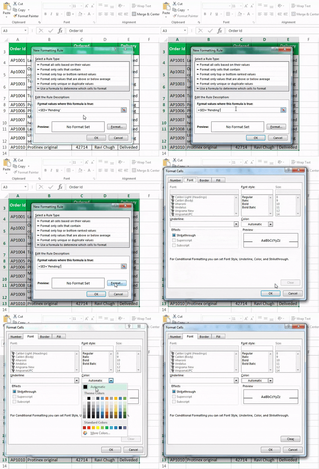
Then click the “FILL” tab, choose a color per our requirement, and click “OK.”

As a result, it will highlight all the rows whose “Delivery Status” is “Pending.”

How Does It Work?

The “Conditional Formatting” option checks each cell in the selected range for the condition or formula.
Our formula is =$E3=“Pending”
As a result, it will analyze each cell in row no 4. It will start from cell A4 and check whether cell E4 has the “Delivery Status” as “Pending” or not. If it does, those rows will get highlighted. Else, it does not.
We have used the $ sign before the column alphabet ($E3), which means that we have locked “Column E,” “Delivery Status,” which we are looking for.
While checking cell A4 for the condition, it will check cell E4.
When cell A5 is checked for the condition, it will check cell E5.
This process will highlight the rows having “Pending” status.

Important Things To Note

This article used text criteria to highlight the row or cells based on another cell value.
Similarly, we can use the other criteria by entering different conditions under the “Formula” text box, depending on our requirements.

Frequently Asked Questions

1. Define Conditional Formatting in Excel.

Conditional formatting in Excel is a feature mainly used for highlighting desired information in a selected dataset or a cell range, based on a single or multiple criterias. It modifies the look of the data to comprehend easily or make the final output presentable.

2. Once applied, how can we remove the Conditional Formatting in Excel?

We can remove the Conditional Formatting in Excel as follows:
• First, choose the entire dataset or the cell range where the Conditional Formatting Rules are created.
• Next, select the “Home” tab - go to the “Styles” group - click the “Conditional Formatting” option drop-down - click the “Clear rules” option right-arrow - select the “Clear Rules from Selected Cells” option, as shown below.

Conditional Formatting - Clear Rules

3. Is there an alternative way to copy the Conditional Formatting in Excel?

An alternate way to copy the Conditional Formatting Rule is by using the “Format Painter”.
• First, select the cells with the Conditional Formatting Rule you want to copy.
• Next, follow the path Home - Clipboard - Format Painter, as shown below.

Download Template

This article must help understand Conditional Formatting based on another cell value with its formulas and examples. You can download the template here to use it instantly.

Conditional Formatting Based On Another Cell Value

What Is Conditional Formatting Based On Another Cell Value?