Table Of Contents
CONCATENATE in Excel
The CONCATENATE function in Excel helps the user concatenate or join two or more cell values which may be in the form of characters, strings or numbers. For example, the formula “=CONCATENATE(A4,“ ”,B4)” joins the cells A4 and B4 containing the values “Rock” and “Band” respectively. It returns the string of cell A4, followed by a space character, and the string of cell B4. Hence, the output is “Rock Band.”
With CONCATENATE, the content of different cells is combined together and placed in a single cell. The CONCATENATE function in Excel acts as a substitute for the “&” operator and joins the values. The usage of the “&” operator makes the formula's complex. In contrast, the CONCATENATE formulas are simple and easy to understand.
Syntax
The syntax of the function is shown in the following image:

The function accepts the following arguments:
- Text1: This is the first cell reference, text value or number to be joined.
- Text2: Thisis the second cell reference, text value or number to be joined.
“Text1” is the required argument. “Text2” and the subsequent arguments are optional and can be added based on the user’s requirement.
Note: The optional arguments are enclosed within the square brackets.
How to Use the CONCATENATE Function in Excel?
Let us understand the working of the CONCATENATE function with the help of the following examples.
Example #1
The following table shows the first and the last names in columns A and B, respectively. We want to join the first name and the last name together so that the full name is displayed in the column C. Use the CONCATENATE function of Excel.
| First Name | Last Name |
|---|---|
| Adam | Cook |
| Albert | Parker |
| Billy | Collins |
| Clark | Rogers |
| Elvis | Cooper |
| Fred | Peterson |
| Sophia | Woods |
| Emma | Barnes |
| Olivia | Ford |
| Emily | Freeman |
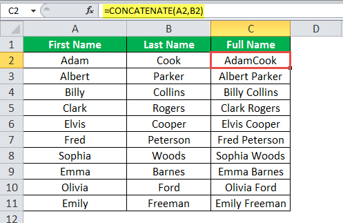
We apply the following CONCATENATE excel formula to join the names of cells A2 and B2:
“=CONCATENATE(A2,B2)”
The output of the formula is shown in cell C2. The first and the last name are joined without a space between them. As a result, the readability of the full name in cell C2 is affected.
To introduce a space between the first and the last names, let us pass another argument to the CONCATENATE formula (between the text values A2 and B2).
The second argument is a string literal with a space enclosed within the double quotes (“ ”).In a string literal, characters exist at their literal value.
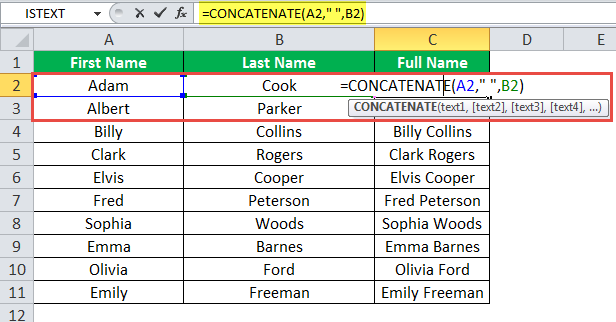
We apply the following formula in cell C2, as shown in the succeeding image.
“=CONCATENATE(A2,“ ”,B2)”
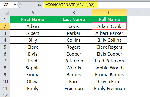
The output is shown in the following image. A space has been inserted between the first and last names in cell C2.
Example #2
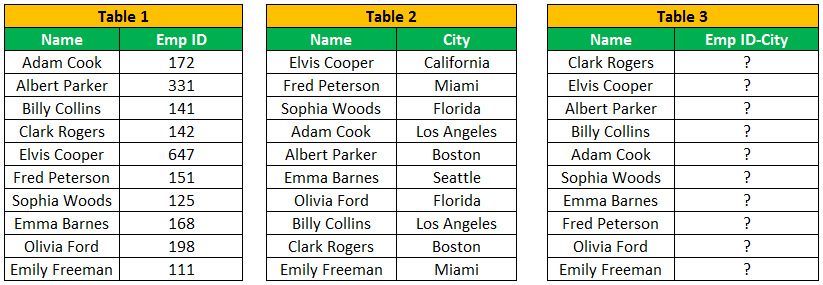
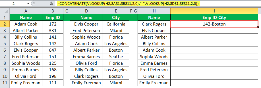
The following image shows three tables titled “table 1,” “table 2,” and “table 3.” All the three tables consist of the names of ten employees of an organization. In addition, “table 1” and “table 2” show the employee IDs and the native places (cities), respectively.
The names of “table 2” and “table 3” are not according to the sequence given in “table 1.”
For every employee, we want to join the IDs and the cities with a hyphen in between. The resulting concatenated values should be listed in the second column of “table 3” which displays question marks.
Since “table 2” and “table 3” do not show the names in the order listed in “table 1,” we cannot pass the reference values directly. Moreover, passing direct values is a time-consuming task which requires the matching of entries.
Instead, let us use the VLOOKUP function to look up the employee ID and the city. The values thus returned can be concatenated.
We apply the following formula to cell I2. The VLOOKUP function is nested within the CONCATENATE excel function.
“=CONCATENATE(VLOOKUP(H2,$A$1:$B$11,2,0),“ -” ,VLOOKUP(H2,$D$1:$E$11,2,0))”
The output of the formula is shown in cell I2 of the following image.
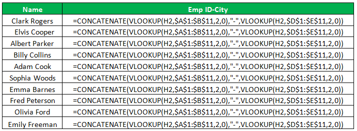
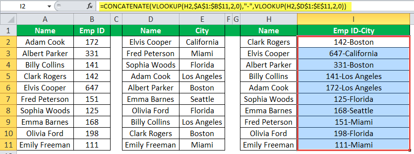
Drag the formula to the remaining cells of column I, as shown in the following image.
The final output is displayed in column I of “table 3.”
Concatenate Excel Function - Video Explanation
The “#NAME” Error in CONCATENATE Excel Function
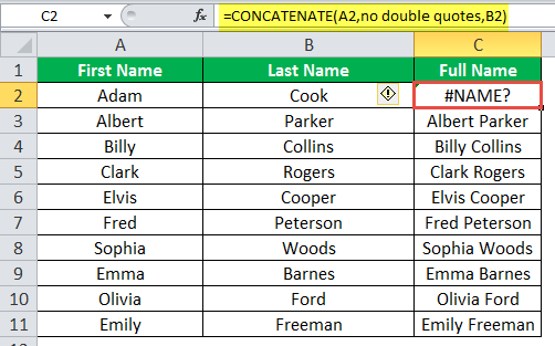
When the user passes an argument apart from the reference value in the formula, it should be enclosed within double quotes. The arguments within the double quotes are the string literals written in the C++ programming language. String literals are used in MS Excel and other office packages.
If the string is not enclosed within double quotes, the CONCATENATE excel function does not recognize it. Hence, it returns the “#NAME” error.
The succeeding image shows the error returned by the CONCATENATE formula in cell C2. This takes place because the second string argument is not enclosed in double quotes.
In the CONCATENATE function, the result of formulas can be concatenated. For this, the different formulas must be passed as an argument to the function.
Limitation of the CONCATENATE Excel Function
With the CONCATENATE excel function, we can combine all the text values of a list into a single string. The function accepts the text values as arguments.
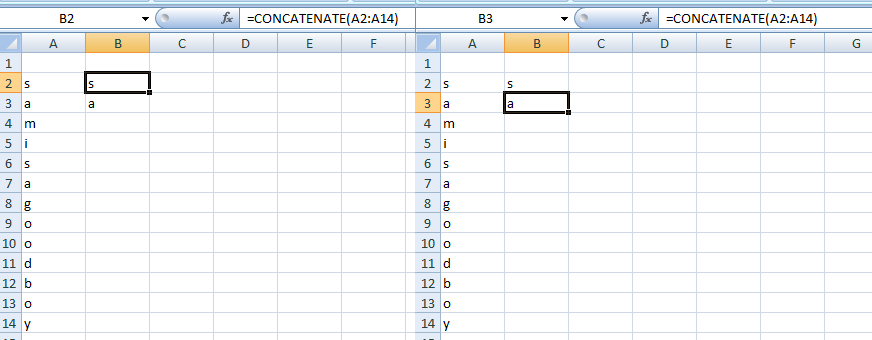
The limitation of the CONCATENATE function is that we cannot pass a range of values as an argument. As a result, the user has to enter individual cell references one by one in the function. This is a time-taking and challenging task for the user.
If we pass a range of values, the CONCATENATE function picks up the cell values of the row to which the formula has been applied. The same is displayed in the following image.
To overcome this limitation, a new function, TEXTJOIN has been introduced in the latest version of the Excel. It concatenates the values on specifying the range (like A2:A14), rather than individual cell references.
The syntax of the TEXTJOIN function is stated as follows:
“=TEXTJOIN(delimiter, ignore_empty, range)”
Where,
- Delimiter: It refers to the separators like “tab,” “semicolon,” “comma,” and “space” used between the values to be combined.
- Ignore_empty: It checks if the empty cells are to be ignored or added to the result. If it returns “true,” the empty cells are ignored. If it returns “false,” the empty cells are included in the result.
- Range: It is the range of values to be concatenated.
All the three arguments “delimiter”, “ignore_empty,” and “range” are mandatory.

