Compound Interest Formula in Excel

Last Updated :

Blog Author :

Edited by :

Reviewed by :

Table Of Contents

Compound Interest in Excel Formula

Compound interest is the addition of interest to the principal sum of a loan or deposit or interest on interest. Rather than paying it out, it is the outcome of reinvesting interest so that interest in the next period is earned on the principal sum plus previously accumulated interest.

For example, suppose you invested $5,000 with a 10% annual interest rate and annually compounded. In such a situation, you may earn $500 ($5,000x10%) as interest from the initial investment(principal). Therefore, from the initial investment, you may earn $5,000+$500= $5,500. Then, in the next period, you may make interest based on the gross amount from the last period. In this example, after two years, from the initial investment, you may earn $550 ($5,500x10%) as your first investment was $5,500. Now, your investment worth will be $5,550.

While simple interest is calculated only on the principal and (unlike compound interest) not on principal plus interest earned or incurred in the previous period.

The total accumulated value, including the principal sum P plus the compounded interest I, is given by the formula:

Where,

P is the original principal sum
P' is the new principal sum
n is the compounding frequency
r is the nominal annual interest rate
t is the overall length of the interest applied (expressed using the same time units as r, usually years).

Compound Interest in Excel Formula

Video Explanation of Compound Interest Examples

How to Calculate Compound Interest in Excel Formula? (with Examples)

Let us understand the same using some examples of the Compound Interest formula in Excel.

Example #1 - Using Mathematical Compound Interest Excel Formula

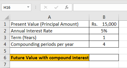
Suppose we have the following information to calculate compound interest in Excel.

As we have described the formula above, we will implement the same in MS Excel using cell references in excel and various operators.

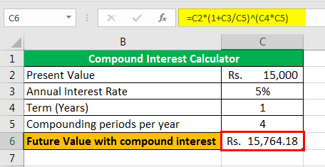
As the C2 cell contains the principal amount (We can also call it as present value). We need to multiply this value with the interest rate.
The interest is to be compounded quarterly (C5), so we need to divide the annual interest rate with cell C5.
As interest is being compounded four times in a year, we need to reference a cell where the number of years is mentioned to multiply 4 with the number of years. That is why the formula would be like this:
After pressing the Enter button, we will get ₹15764.18 as the future value with compound interest.

It is like a compound interest calculator in Excel now. We can change the value for the annual interest rate, the number of years, and compounding periods per year as below.

Example #2 - Using the Compound Interest Calculation Table in Excel

Suppose we have the following information to calculate compound interest in a table excel format (systematically).

Step 1 - We need to name cell E3 "Rate" by selecting the cell and changing the name using the "Name Box."

Step 2 - We have the principal value or present value as ₹15,000, and the annual interest rate is 5%. To calculate the investment value at the end of quarter 1, we will add 5%/4, i.e., 1.25% interest, to the principal value.

The result is shown below:

Step 3 - We must drag the formula to the C6 cell by selecting the range C3:C6 and pressing "Ctrl+D."

The future value after four quarters will be ₹15764.18.

Example #3 - Compound Interest Using FVSCHEDULE Excel Formula

Suppose we have the following information to calculate compound interest in Excel.

We will use the FVSCHEDULE function to calculate future value. The FVSCHEDULE formula returns the future value of an initial principal after applying a series of compound interest rates.

To do the same, the steps are:

Step 1 - We will initiate writing the FVSCHEDULE function into cell B6. The function takes two arguments, i.e., principal and schedule.

We need to give the amount we are investing in for the principal.
We need to provide the list of interest rates with commas in curly braces for the schedule to calculate the value with compound interest.

Step 2 - For 'principal,' we will provide the reference of the B1 cell, and for 'schedule,' we will specify 0.0125 as this is the value we get when we divide the 5% with 4.

The result is shown below:

Now, we can apply the FVSCHEDULE formula in Excel.

Step 3 - After pressing the Enter button, we get ₹15764.18 as the future value with compound interest in Excel.

Example #4 - Compound Interest Using the FV Excel Formula

Suppose we have the following data to calculate compound interest in Excel.

We will use the FV Excel formula to calculate compound interest.

FV function (stands for Future Value) returns the future value of an investment based on periodic, constant payments and a constant interest rate.

The syntax of the FV function is

The argument in the FV function is:

Rate: Rate is the constant interest rate per period in an annuity.
Nper: Nper stands for the total number of periods in an annuity.
Pmt: PMT stands for payment. It indicates the amount we will add to the annuity every period. If we omit this value, then it is mandatory to mention PV.
PV: PV stands for present value. It is the amount which we are investing in. This amount is going out of our pocket, so by convention, this amount is mentioned with a negative sign.
Type: This is an optional argument. We need to specify 0 if the amount is being added to the investment at the end of the period or one if the amount is being added to the investment at the beginning of the period.

We need to mention either the PMT or PV argument.

We will specify the rate as "Annual Interest Rate (B2)/ Compounding periods per year (B4)."

We need to specify nper as 'Term (Years) * Compounding periods per year.'

As we will not add any additional amount to the principal value during the investment period, we will specify '0' for "pmt."

We have omitted the value for "pmt," and we are investing ₹15,000 as principal (present value). We will reference the B1 cell with a negative sign for "PV."

After pressing the "Enter" button, we get ₹15764.18 as the future value with compound interest.

Things to Remember about Compound Interest Formula in Excel

We need to insert the interest rate in percentage form (4%) or decimal form (0.04).
As the "PMT" and "PV" arguments in the FV function outflows, in reality, we need to mention them in the negative form (with a minus (-) sign).
FV function gives #VALUE! Error when any non-numeric value is provided as an argument.
We need to mention either PMT or PV arguments in the FV function.