Compare Two Columns in Excel

Last Updated :

Blog Author :

Edited by :

Reviewed by :

Table Of Contents

Compare two Columns in Excel

Two columns in excel are compared when their entries are studied for similarities and differences. The similarities are the data values that exist in the same row of both the compared columns. In contrast, the differences are those values that exist in only one of these columns.

For example, for a specific month, a table displays the following information:

Column A lists the names of the employees who took three consecutive leaves.
Column B lists the names of the employees who took two consecutive leaves.

Since the data pertains to the same organization, there can be a similarity or a difference within the given set of values. The same is explained as follows:

A similarity or a match (column A is equal to column B) implies employees who took both three and two continuous leaves.
A difference (column A is not equal to column B) implies employees who took either three or two continuous leaves.

It is difficult to scan through the data to track the matches and the differences manually. Hence, there are techniques which can be followed to compare 2 columns of an excel worksheet.

Compare two Columns in Excel

How to Compare two Columns in Excel? (Top 4 Methods)

The top four methods to compare 2 columns are listed as follows:

Method #1–Compare using simple formulae
Method #2–Compare using the IF formula
Method #3–Compare using the EXACT formula
Method #4–Compare using conditional formatting

Let us understand these methods with the help of examples.

#1 - Compare Using Simple Formulae

The following table shows the names of the employees of an organization in column A. Columns B and C display their log-in and the log-out times respectively.

We want to compare two excel columns B and C to find out the employees who forgot to logout from the office. The official timings are 10:30 a.m.-7:30 p.m. Use the formula method for comparison.

For the given data, if the log-in time is equal to the log-out time, we assume that the employee has forgotten to logout.

The steps to compare two columns in excel with the help of the comparison operator “equal to” (=) are listed as follows:

In cell D2, enter the symbol “=” followed by selecting the cell B2.
Enter the symbol “=” again, followed by selecting the cell C2.
Press the “Enter” key. It returns “false.” This implies that the value in cell B2 is not equal to that of cell C2.
Drag or copy-paste the formula to the remaining cells. The output is either “true” or “false,” as shown in the following image.
If the value in column B is equal to that of column C, the result is “true,” else “false.” The cells D5 and D9 show the output “true.”
Hence, Roshan and Uday forgot to logout from the office.

#2 - Compare 2 Columns Using the IF Formula

Working on the data of example #1, we want the following results:

“Forgot to punch out,” if the employee forgets to logout
“No problem,” if the employee logs out

Use the IF function to compare the columns B and C.

We apply the following formula.

“=IF(B2=C2,“Forgot to Punch Out”,“No Problem”)”

If the value in column B is equal to that of column C, the result is “true,” otherwise “false.” For every “true” value, the formula returns “forgot to punch out.” Likewise, it returns “no problem” for every “false” value.

The output is shown in column E of the following image.

Hence, Roshan and Uday are the only two employees who have forgotten to logout from the office.

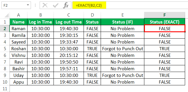
#3 - Compare Using the EXACT Formula

Working on the data of example #1, we want to compare the two excel columns B and C with the help of the EXACT function.

We apply the following formula.

“=EXACT(B2,C2)”

If the value in column B is equal to that of column C, the formula returns “true,” otherwise “false.” The output is shown in column F of the following image.

Hence, the entries of columns B and C are identical for Roshan and Uday.

Note: The EXACT function is case-sensitive.

We have written the name “Raman” in columns A and B with different casing. We apply the following formula.

“=EXACT(A2,B2)”

The formula returns “false” when the casing of cell A2 is different from that of cell B2. Likewise, it returns “true” if the casing in columns A and B is the same.

The output is shown in column C of the following image.

#4 - Compare 2 Excel Columns Using Conditional Formatting

Working on the data of example #1, we want to highlight those entries that are identical in columns B and C. Use the conditional formatting feature.

Step 1: Select the entire data. In the Home tab, click the “conditional formatting” drop-down under the “styles” section. Select “new rule.”

Step 2: The “new formatting rule” window appears. Under “select a rule type,” choose the option “use a formula to determine which cells to format.”

Step 3: Enter the formula “$B2=$C2” under “edit the rule description.”

Step 4: Click “format.” In the “format cells” window, select the color to highlight the identical entries. Click “Ok.” Click “Ok” again in the “new formatting rule” window.

Step 5: The matches of columns B and C are highlighted, as shown in the following image.

Hence, the entries of columns B and C are identical for Roshan and Uday.

The Properties of the Comparison Methods

The features of the comparison methods discussed are listed as follows:

The outcomes of the IF function can be modified according to the requirement of the user.
The EXACT function returns “false” for two same values having different casing.
The simplest technique to compare two excel columns is by using the comparison operator “equal to” (method #1).

Note: The comparison method to be used depends on the data structure and the kind of output required.

Frequently Asked Questions

1. What does it mean to compare two columns and how is it done in Excel?

The comparison of two data columns helps find the similarities and the differences. In case of similarity, a value exists in the same row of both the columns. In contrast, a difference is a deviation of one value from the other.

To compare two excel columns, the easiest approach is listed as follows:
a. Enter the following formula.
“=cell1=cell2”
The “cell1” is a cell containing a data value in the first column. The “cell2” is a cell containing a data value in the second column. Both “cell1” and “cell2” are in the same row.
b. Press the “Enter” key.
The formula returns “true” or “false” depending on whether the value exists in both the compared columns or not.

2. How to highlight the different values of two columns without using the formula in Excel?

Let us compare the following 2 columns consisting of names in the mentioned sequence:
• Column A contains Jack, Adam, Elizabeth, Betty, and Veronica.
• Column B contains Robert, Peter, Elizabeth, Henry, and Veronica.

The steps to highlight the different values without using the formula are listed as follows:

a. Select columns A and B.
b. In the Home tab, click “find and select” drop-down under the “editing” group. Choose “go to special.”
c. In the “go to special” window, select “row differences.” Click “Ok.”

The names Robert, Peter, and Henry of column B are highlighted. These cells can be colored using the “fill color” property of Excel.

3. How to compare multiple columns in Excel?

Let us compare the following columns consisting of numbers in the mentioned sequence:

• Column A contains 3, 49, 20, 22, and 86 in the range A1:A5.
• Column B contains 29, 49, 38, 21, and 86 in the range B1:B5.
• Column C contains 12, 49, 56, 24, and 86 in the range C1:C5.

The steps to compare columns A, B, and C are stated as follows:

a. Enter the following formula in cell D1. “IF(COUNTIF($A1:$C5,$A1)=3,“full match”,“”)”
b. Press the “Enter” key.
c. Drag or copy-paste the formula to the remaining cells.

Since we are comparing three excel columns, we enter the number 3 in the formula. The formula returns “full match” in cells D2 and D5. It returns an empty string in the cells D1, D3, and D4.

Hence, the numbers 49 and 86 appear in the respective rows 2 and 5 of all the three columns.