Columns Function in Excel

The COLUMNS function is a built-in function in Microsoft Excel. It falls under the category of LOOKUP functions in Excel. The COLUMNS function returns the total number of columns in the given array or collection of references. The purpose of the COLUMNS formula in Excel is to know the number of columns in an array of references.

For example, the formula =COLUMNS(A1:E3) will return as 5 since the range A1:E3 has 5 columns, A, B, C, D, and E, respectively.

• The COLUMNS function in excel is used to find the number of columns used in the worksheet.
• The formula of the columns function in excel is =COLUMN(array), where the array is the only mandatory argument.
• The array shows the range of cells for which the number of columns is derived.
• We can choose either a single cell or a range as the value in the array argument.
• It is important to know that the function will return only the number of columns even if the chosen array has multiple rows and columns.

• array = This is a required parameter. An array / a formula resulting in an array / a reference to a range of Excel cells for which the number of columns is to be calculated.

The COLUMNS function has only one argument, and it is mandatory.

The said function is a worksheet (WS) function. As a WS function, columns can be inserted as a part of the formula in a worksheet cell.

Let us look at the examples given below to understand the use of the COLUMNS function in excel.

Example #1 – Total Columns In A Range

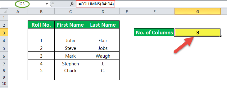
In the example of this column, cell G3 has a formula associated with it. So, G3 is a result cell.

The argument for the COLUMNS function in excel is a cell range, which is B4:D4. Here, B4 is a starting cell, and D4 is the ending cell.

The number of columns between these two cells is 3. So, the result is 3.

Example #2 – Total Cells In A Range

In this example, cell G4 has a formula associated with it. So, G4 is a result cell.

The formula is COLUMNS (B4: E8) * ROWS*B4: E8). Then, multiplication is performed between the total number of columns and a total number of rows for the given range of cells in the sheet.

Here, the total number of columns is four, and the total number of rows is 5. So, the total number of cells is 4*5 = 20.

Example #3 – Get The Address Of The First Cell In A Range

Here, the dataset is named data. Further, this data is used in the formula.

You may refer to the steps given below to name the dataset.

• Step 1: Select the cells.
• Step 2: Right-click and choose Define Name.
• Step 3: Name the dataset as data.

In the example of these columns, cell G6 has a formula associated with it. So, G6 is a result cell. The formula is to calculate the first cell in the dataset represented by the name data. The result is $B$4, i.e., B4, the last cell in the selected dataset.

The formula uses the ADDRESSES function, which has two parameters: row number and column number.

E.g., ADDRESS (8,5) returns $B$4. Here, 4 is the row number, and 2 is the column number. So, the function returns a cell denoted by these row and column numbers.

Here, a row number is calculated by

ROW(data)

And the column number is calculated by

COLUMN(data)

Example 4 – Get The Address Of The Last Cell In A Range

Here, the dataset is named data. Further, this data is used in the column’s formula in Excel. We can refer to the steps given below to name the dataset.

• Step 1: Select the cells.
• Step 2: Right-click and choose Define Name.
• Step 3: Name the dataset as data.

In this COLUMNS example, cell G5 has a formula associated with it. So, G5 is a result cell. The formula is to calculate the last cell in the dataset represented by the name data. The result is $E$8, i.e., E8, the last cell in the selected dataset.

The formula uses the ADDRESSES function, which has two parameters: row number and column number.

E.g., ADDRESS (8,5) returns $E$8. Here, 8 is the row number, and 5 is the column number. So, the function returns a cell denoted by these row and column numbers.

Here, the row number is calculated by

ROW(data)+ROWS(data-1)

And the column number is calculated by

COLUMN(data)+COLUMNS(data-1)

• The argument of the COLUMNS function in Excel can be a single cell address or a range of cells.
• The argument of the COLUMNS function cannot point to multiple references or cell addresses.

This article is a guide to Columns Function in Excel. We discuss the columns formula in Excel and how to use it, along with examples and downloadable templates. You can also go through our other suggested articles: -

• Excel Column Lock
• Excel Freeze Columns
• Group Column in Excel
• Column in Excel
• Break Links in Excel