Table Of Contents
What Is Excel Column Merge?
Column Merge in Excel merges cell values in two or more cells in Excel. We must use the formula in every column cell by dragging or copy-paste the formula in each column.
Excel Column Merge can be performed using the ampersand (&) and the CONCAT function in Excel.
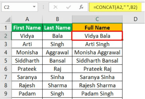
For example, we have a list of candidates with the first name in one column and the last name in another. The requirement here is to get the full name of all candidates in one column. We can do this using the Column Merge in Excel.
Key Takeaways
- Column Merge in Excel helps users to combine or merge 2 or more cell values like first, middle, or last names, or Names with employee IDs, or names with respective locations.
- We use the Ampersand (&) and CONCAT() ways to combine cell values and display the results. We can also use the delimiters, such as space, comma, dot, hyphen, etc.
- The CONCAT function works with Excel 2016 or later versions. If we are working on the earlier version of Excel, we can use the CONCATENATE function.
How To Merge Multiple Columns In Excel?
We can merge the cells using two ways.
- Using the CONCAT Function.
- Merge the Cells by Using the “&” Symbol.
Examples
We will consider specific examples for the above-mentioned methods.
Example #1 – Using the CONCAT Function
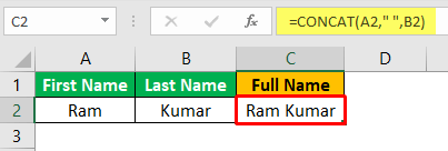
We have Ram and Kumar in the last name column in the first name column. Now, we need to merge the value in the full name column. So here we use =CONCAT(A2,“ ”,B2). The result is shown below.

We have noticed that we have used double-quotes (“ ”) between the A2 and B2. That is used to give space between the first and the last name. If use double-quotes without space as “” in the function, then the result will be Ramkumar.
Example #2 – Merge the Cells by Using the “&” Symbol
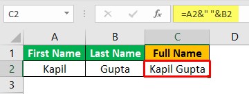
In the following image, we will merge the cells using the “&” symbol with the CONCAT function.

We can merge the cells using the “&” symbol in the formula. So, the formula will be =A2&“ ”&B2. The result is Kapil Gupta, as shown below.
Let us merge the value into two columns.
Example #3
We have a list of first and last names in two columns, A and B, as shown in the image below. Now, we require the full name in column C.

Follow the below steps:
- First, select cell C2.
- Then, insert the formula =CONCAT(A2,“ ”,B2), and press “Enter”.
- Next, drag the formula from cell C2 to C11 using the fill handle, i.e., if we have the first name and last name till the 11th row, then paste the formula till C11.
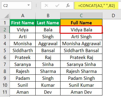
The output is shown above.
Example #4
Suppose we have a list of 10 students whose first, middle, and last names are in columns A, B, and C, and we need the full name in column D.
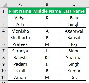
Follow the below steps:
- First, select cell D2.
- Then, insert the formula =CONCAT(A2,“ ”,B2,“ ”,C2), and press “Enter”.
- Next, drag the formula from cell D2 to D11 using the fill handle, i.e., if we have the first, middle, and the last names till the 11th row, then paste the formula till D11.
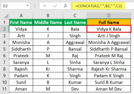
The output is shown above.
Example #5
We have a list of first and last names in two columns, A and B, below. Next, we need to create a user ID for each person.
Note: Space is not allowed in a user ID.

Follow the below steps:
- First, select cell C2.
- Then, insert the formula =CONCAT(A2,“.”,B2), and press “Enter”.
- Next, drag the formula from cell C2 to C11 using the fill handle, i.e., if we have the first and the last name till the 11th row, then paste the formula till C11.
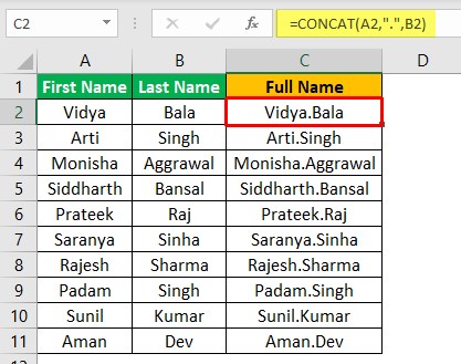
The output is shown above. Similarly, we can merge the value using some other character, i.e., (dot (.), hyphen (-), the asterisk (*), etc.
Important Things To Note
- CONCAT function works with Excel 2016 or above version. If we are working on the earlier version of Excel, we need to use the CONCATENATE function.
- It is not mandatory to use any space or special character while merging the cells. We can merge the cells in excel or columns without using anything.
