Column Function in Excel

The column function in Excel is used to determine the column numbers of the target cells. Although it is also a built-in worksheet function and takes only one argument, the target cell, as a reference, notes that this function does not provide the cell's value as it returns only the column number of the cell. In simple words, this Excel column formula will give a numeric value as output which signifies the column number of the supplied reference.

For example, the formula COLUMN(A4) returns 1 since COLUMN A is the first column in the Excel worksheet.

Optional parameter:

• : The reference parameter is optional. If we do not supply the reference to this function, it will return the current column number where the function is located.

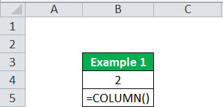
Example #1

As shown below, the column function provides the column number of the current cells where the column formula is located if the reference is excluded or omitted.

Example #2

If the range C5 is supplied to the column function in Excel, it will return column number 3 as output.

Example #3

If a range is supplied to the column function as input, it will return the first column number as output for the below table. The output will be 3.

Example #4

The column function with VLOOKUP function in Excel.

We can use the column function with other functions. For example, we are using this function with the lookup function here.

Suppose we have employee data containing ID, name, and salary column. And we have to find out the name from the ID. Then, we can use the VLOOKUP function combined with this function, as shown below.

=VLOOKUP(B11,$B$11:$D$15,COLUMN(C11),0)

Example #5

The column function with MOD function.

Suppose a cable connection expense that is payable every third month. The cable connection expense amount is $50. We can use the column formula with the MOD function below to generate a fixed value every third month.

The column formula used is =IF(MOD(COLUMN(B8)-1,3)=0,$A$2,0), as shown below:

Example #6

Suppose we need to obtain the address of the first cell in a supplied range. So, here, we can use the ADDRESS function with ROW and COLUMN. The column formula in excel to be used is below:

=ADDRESS(ROW(B24:D24)+ROWS(B24:D24)-1,COLUMN(B24:D24)+COLUMNS(B24:D24)-1)

This column formula in Excel returns the ADDRESS of the first cell based on a row and column number. Here, we use the ROW function to generate a list of row numbers and then add ROWS(B5: D5)-1 to ROW(B24: D24) so that the first item in the array is the last row number.

Then we do the same for COLUMN and COLUMNS: COLUMN(B24:D24)+COLUMNS(B24:D24)-1)

After applying this function, it can return an array of addresses. For example, if we enter the column formula in a single cell, we get the item ($D$24) from the array/range, the address corresponding to the last cell in a range, as shown below.

Example #7

Suppose we have to find out the last column in a range. We can use the MIN function in Excel. The details are as follows:

=MIN(COLUMN(B23:D26))+COLUMNS(B23:D26)-1

If we provide a single cell as a reference to the COLUMN, it will return the column number as output for that particular reference/cell. However, when we supply a range with multiple columns, this function may give an array as output containing all column numbers for the given range. Therefore, if we want to get only the first column number as output, we must use the MIN function to get the first column number, the lowest number in the array. The result is shown below:

• This function will return a #NAME! Error if we supply the invalid reference.